


1. 可视化网络结构
在复杂的网络结构中确定每一层的输入结构,方便我们在短时间内完成debug
1.1 使用print函数打印模型基础信息
使用ResNet18的结构进行展示
import torchvision.models as models
model = models.resnet18()
print(model)

#打印结果
ResNet(
  (conv1): Conv2d(3, 64, kernel_size=(7, 7), stride=(2, 2), padding=(3, 3), bias=False)
  (bn1): BatchNorm2d(64, eps=1e-05, momentum=0.1, affine=True, track_running_stats=True)
  (relu): ReLU(inplace=True)
  (maxpool): MaxPool2d(kernel_size=3, stride=2, padding=1, dilation=1, ceil_mode=False)
  (layer1): Sequential(
    (0): Bottleneck(
      (conv1): Conv2d(64, 64, kernel_size=(1, 1), stride=(1, 1), bias=False)
      (bn1): BatchNorm2d(64, eps=1e-05, momentum=0.1, affine=True, track_running_stats=True)
      (conv2): Conv2d(64, 64, kernel_size=(3, 3), stride=(1, 1), padding=(1, 1), bias=False)
      (bn2): BatchNorm2d(64, eps=1e-05, momentum=0.1, affine=True, track_running_stats=True)
      (conv3): Conv2d(64, 256, kernel_size=(1, 1), stride=(1, 1), bias=False)
      (bn3): BatchNorm2d(256, eps=1e-05, momentum=0.1, affine=True, track_running_stats=True)
      (relu): ReLU(inplace=True)
      (downsample): Sequential(
        (0): Conv2d(64, 256, kernel_size=(1, 1), stride=(1, 1), bias=False)
        (1): BatchNorm2d(256, eps=1e-05, momentum=0.1, affine=True, track_running_stats=True)
      )
    )
   ... ...
  )
  (avgpool): AdaptiveAvgPool2d(output_size=(1, 1))
  (fc): Linear(in_features=2048, out_features=1000, bias=True)
)
1.2 使用torchinfo可视化网络结构
1.2.1 torchinfo的安装
# 安装方法一
pip install torchinfo
# 安装方法二
conda install -c conda-forge torchinfo
1.2.2 torchinfo的使用
(1)方法:torchinfo.summary()
(2)参数:(这里展示的是函数定义时传入的参数),具体请看参数详解)
def summary(
    model: nn.Module,
    input_size: Optional[INPUT_SIZE_TYPE] = None,
    input_data: Optional[INPUT_DATA_TYPE] = None,
    batch_dim: Optional[int] = None,
    cache_forward_pass: Optional[bool] = None,
    col_names: Optional[Iterable[str]] = None,
    col_width: int = 25,
    depth: int = 3,
    device: Optional[torch.device] = None,
    dtypes: Optional[List[torch.dtype]] = None,
    mode: str | None = None,
    row_settings: Optional[Iterable[str]] = None,
    verbose: int = 1,
    **kwargs: Any,
) -> ModelStatistics
(3)实例以ResNet18为例:
import torchvision.models as models
from torchinfo import summary
resnet18 = models.resnet18() # 实例化模型
summary(resnet18, (1, 3, 224, 224)) # 1:batch_size 3:图片的通道数 224: 图片的高宽


# 结果输出
=========================================================================================
Layer (type:depth-idx)                   Output Shape              Param #
=========================================================================================
ResNet                                   --                        --
├─Conv2d: 1-1                            [1, 64, 112, 112]         9,408
├─BatchNorm2d: 1-2                       [1, 64, 112, 112]         128
├─ReLU: 1-3                              [1, 64, 112, 112]         --
├─MaxPool2d: 1-4                         [1, 64, 56, 56]           --
├─Sequential: 1-5                        [1, 64, 56, 56]           --
│    └─BasicBlock: 2-1                   [1, 64, 56, 56]           --
│    │    └─Conv2d: 3-1                  [1, 64, 56, 56]           36,864
│    │    └─BatchNorm2d: 3-2             [1, 64, 56, 56]           128
│    │    └─ReLU: 3-3                    [1, 64, 56, 56]           --
│    │    └─Conv2d: 3-4                  [1, 64, 56, 56]           36,864
│    │    └─BatchNorm2d: 3-5             [1, 64, 56, 56]           128
│    │    └─ReLU: 3-6                    [1, 64, 56, 56]           --
│    └─BasicBlock: 2-2                   [1, 64, 56, 56]           --
│    │    └─Conv2d: 3-7                  [1, 64, 56, 56]           36,864
│    │    └─BatchNorm2d: 3-8             [1, 64, 56, 56]           128
│    │    └─ReLU: 3-9                    [1, 64, 56, 56]           --
│    │    └─Conv2d: 3-10                 [1, 64, 56, 56]           36,864
│    │    └─BatchNorm2d: 3-11            [1, 64, 56, 56]           128
│    │    └─ReLU: 3-12                   [1, 64, 56, 56]           --
├─Sequential: 1-6                        [1, 128, 28, 28]          --
│    └─BasicBlock: 2-3                   [1, 128, 28, 28]          --
│    │    └─Conv2d: 3-13                 [1, 128, 28, 28]          73,728
│    │    └─BatchNorm2d: 3-14            [1, 128, 28, 28]          256
│    │    └─ReLU: 3-15                   [1, 128, 28, 28]          --
│    │    └─Conv2d: 3-16                 [1, 128, 28, 28]          147,456
│    │    └─BatchNorm2d: 3-17            [1, 128, 28, 28]          256
│    │    └─Sequential: 3-18             [1, 128, 28, 28]          8,448
│    │    └─ReLU: 3-19                   [1, 128, 28, 28]          --
│    └─BasicBlock: 2-4                   [1, 128, 28, 28]          --
│    │    └─Conv2d: 3-20                 [1, 128, 28, 28]          147,456
│    │    └─BatchNorm2d: 3-21            [1, 128, 28, 28]          256
│    │    └─ReLU: 3-22                   [1, 128, 28, 28]          --
│    │    └─Conv2d: 3-23                 [1, 128, 28, 28]          147,456
│    │    └─BatchNorm2d: 3-24            [1, 128, 28, 28]          256
│    │    └─ReLU: 3-25                   [1, 128, 28, 28]          --
├─Sequential: 1-7                        [1, 256, 14, 14]          --
│    └─BasicBlock: 2-5                   [1, 256, 14, 14]          --
│    │    └─Conv2d: 3-26                 [1, 256, 14, 14]          294,912
│    │    └─BatchNorm2d: 3-27            [1, 256, 14, 14]          512
│    │    └─ReLU: 3-28                   [1, 256, 14, 14]          --
│    │    └─Conv2d: 3-29                 [1, 256, 14, 14]          589,824
│    │    └─BatchNorm2d: 3-30            [1, 256, 14, 14]          512
│    │    └─Sequential: 3-31             [1, 256, 14, 14]          33,280
│    │    └─ReLU: 3-32                   [1, 256, 14, 14]          --
│    └─BasicBlock: 2-6                   [1, 256, 14, 14]          --
│    │    └─Conv2d: 3-33                 [1, 256, 14, 14]          589,824
│    │    └─BatchNorm2d: 3-34            [1, 256, 14, 14]          512
│    │    └─ReLU: 3-35                   [1, 256, 14, 14]          --
│    │    └─Conv2d: 3-36                 [1, 256, 14, 14]          589,824
│    │    └─BatchNorm2d: 3-37            [1, 256, 14, 14]          512
│    │    └─ReLU: 3-38                   [1, 256, 14, 14]          --
├─Sequential: 1-8                        [1, 512, 7, 7]            --
│    └─BasicBlock: 2-7                   [1, 512, 7, 7]            --
│    │    └─Conv2d: 3-39                 [1, 512, 7, 7]            1,179,648
│    │    └─BatchNorm2d: 3-40            [1, 512, 7, 7]            1,024
│    │    └─ReLU: 3-41                   [1, 512, 7, 7]            --
│    │    └─Conv2d: 3-42                 [1, 512, 7, 7]            2,359,296
│    │    └─BatchNorm2d: 3-43            [1, 512, 7, 7]            1,024
│    │    └─Sequential: 3-44             [1, 512, 7, 7]            132,096
│    │    └─ReLU: 3-45                   [1, 512, 7, 7]            --
│    └─BasicBlock: 2-8                   [1, 512, 7, 7]            --
│    │    └─Conv2d: 3-46                 [1, 512, 7, 7]            2,359,296
│    │    └─BatchNorm2d: 3-47            [1, 512, 7, 7]            1,024
│    │    └─ReLU: 3-48                   [1, 512, 7, 7]            --
│    │    └─Conv2d: 3-49                 [1, 512, 7, 7]            2,359,296
│    │    └─BatchNorm2d: 3-50            [1, 512, 7, 7]            1,024
│    │    └─ReLU: 3-51                   [1, 512, 7, 7]            --
├─AdaptiveAvgPool2d: 1-9                 [1, 512, 1, 1]            --
├─Linear: 1-10                           [1, 1000]                 513,000
=========================================================================================
Total params: 11,689,512
Trainable params: 11,689,512
Non-trainable params: 0
Total mult-adds (G): 1.81
=========================================================================================
Input size (MB): 0.60
Forward/backward pass size (MB): 39.75
Params size (MB): 46.76
Estimated Total Size (MB): 87.11
=========================================================================================
2. CNN可视化
卷积神经网路——CNN
2.1 CNN卷积核可视化
以torchvision自带的VGG11模型为例。
import torch
from torchvision.models import vgg11

model = vgg11(pretrained=True)
print(dict(model.features.named_children()))


# 输出
{'0': Conv2d(3, 64, kernel_size=(3, 3), stride=(1, 1), padding=(1, 1)),
 '1': ReLU(inplace=True),
 '2': MaxPool2d(kernel_size=2, stride=2, padding=0, dilation=1, ceil_mode=False),
 '3': Conv2d(64, 128, kernel_size=(3, 3), stride=(1, 1), padding=(1, 1)),
 '4': ReLU(inplace=True),
 '5': MaxPool2d(kernel_size=2, stride=2, padding=0, dilation=1, ceil_mode=False),
 '6': Conv2d(128, 256, kernel_size=(3, 3), stride=(1, 1), padding=(1, 1)),
 '7': ReLU(inplace=True),
 '8': Conv2d(256, 256, kernel_size=(3, 3), stride=(1, 1), padding=(1, 1)),
 '9': ReLU(inplace=True),
 '10': MaxPool2d(kernel_size=2, stride=2, padding=0, dilation=1, ceil_mode=False),
 '11': Conv2d(256, 512, kernel_size=(3, 3), stride=(1, 1), padding=(1, 1)),
 '12': ReLU(inplace=True),
 '13': Conv2d(512, 512, kernel_size=(3, 3), stride=(1, 1), padding=(1, 1)),
 '14': ReLU(inplace=True),
 '15': MaxPool2d(kernel_size=2, stride=2, padding=0, dilation=1, ceil_mode=False),
 '16': Conv2d(512, 512, kernel_size=(3, 3), stride=(1, 1), padding=(1, 1)),
 '17': ReLU(inplace=True),
 '18': Conv2d(512, 512, kernel_size=(3, 3), stride=(1, 1), padding=(1, 1)),
 '19': ReLU(inplace=True),
 '20': MaxPool2d(kernel_size=2, stride=2, padding=0, dilation=1, ceil_mode=False)}
2.2 CNN特征图可视化方法
在PyTorch中,提供了一个专用的接口使得网络在前向传播过程中能够获取到特征图,这个接口的名称非常形象,叫做hook.
首先实现了一个hook类,之后在plot_feature函数中,将该hook类的对象注册到要进行可视化的网络的某层中。model在进行前向传播的时候会调用hook的__call__函数,我们也就是在那里存储了当前层的输入和输出。
class Hook(object):
    def __init__(self):
        self.module_name = []
        self.features_in_hook = []
        self.features_out_hook = []

    def __call__(self,module, fea_in, fea_out):
        print("hooker working", self)
        self.module_name.append(module.__class__)
        self.features_in_hook.append(fea_in)
        self.features_out_hook.append(fea_out)
        return None


def plot_feature(model, idx, inputs):
    hh = Hook()
    model.features[idx].register_forward_hook(hh)

    # forward_model(model,False)
    model.eval()
    _ = model(inputs)
    print(hh.module_name)
    print((hh.features_in_hook[0][0].shape))
    print((hh.features_out_hook[0].shape))

    out1 = hh.features_out_hook[0]

    total_ft  = out1.shape[1]
    first_item = out1[0].cpu().clone()

    plt.figure(figsize=(20, 17))


    for ftidx in range(total_ft):
        if ftidx > 99:
            break
        ft = first_item[ftidx]
        plt.subplot(10, 10, ftidx+1)

        plt.axis('off')
        #plt.imshow(ft[ :, :].detach(),cmap='gray')
        plt.imshow(ft[ :, :].detach())
2.3 CNN class activation map可视化方法
2.3.1 实现方法
CAM系列操作的实现可以通过开源工具包pytorch-grad-cam来实现。
2.3.2 安装
pip install grad-cam2.3.3 例子
import torch
from torchvision.models import vgg11,resnet18,resnet101,resnext101_32x8d
import matplotlib.pyplot as plt
from PIL import Image
import numpy as np
model = vgg11(pretrained=True)
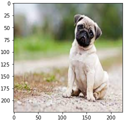
img_path = './dog.png'
# resize操作是为了和传入神经网络训练图片大小一致
img = Image.open(img_path).resize((224,224))
# 需要将原始图片转为np.float32格式并且在0-1之间
rgb_img = np.float32(img)/255
plt.imshow(img)
##########################################################################
from pytorch_grad_cam import GradCAM,ScoreCAM,GradCAMPlusPlus,AblationCAM,XGradCAM,EigenCAM,FullGrad
from pytorch_grad_cam.utils.model_targets import ClassifierOutputTarget
from pytorch_grad_cam.utils.image import show_cam_on_image
target_layers = [model.features[-1]]
# 选取合适的类激活图,但是ScoreCAM和AblationCAM需要batch_size
cam = GradCAM(model=model,target_layers=target_layers)
targets = [ClassifierOutputTarget(preds)]
# 上方preds需要设定,比如ImageNet有1000类,这里可以设为200
grayscale_cam = cam(input_tensor=img_tensor, targets=targets)
grayscale_cam = grayscale_cam[0, :]
cam_img = show_cam_on_image(rgb_img, grayscale_cam, use_rgb=True)
print(type(cam_img))
Image.fromarray(cam_img)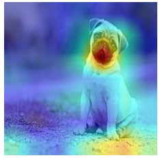
2.4 使用FlashTorch快速实现CNN可视化
2.4.1 安装
pip install flashtorch2.4.2 可视化梯度
# Download example images
# !mkdir -p images
# !wget -nv \
#    https://github.com/MisaOgura/flashtorch/raw/master/examples/images/great_grey_owl.jpg \
#    https://github.com/MisaOgura/flashtorch/raw/master/examples/images/peacock.jpg   \
#    https://github.com/MisaOgura/flashtorch/raw/master/examples/images/toucan.jpg    \
#    -P /content/images

import matplotlib.pyplot as plt
import torchvision.models as models
from flashtorch.utils import apply_transforms, load_image
from flashtorch.saliency import Backprop

model = models.alexnet(pretrained=True)
backprop = Backprop(model)

image = load_image('/content/images/great_grey_owl.jpg')
owl = apply_transforms(image)

target_class = 24
backprop.visualize(owl, target_class, guided=True, use_gpu=True)
2.4.3 可视化卷积核
import torchvision.models as models
from flashtorch.activmax import GradientAscent

model = models.vgg16(pretrained=True)
g_ascent = GradientAscent(model.features)

# specify layer and filter info
conv5_1 = model.features[24]
conv5_1_filters = [45, 271, 363, 489]

g_ascent.visualize(conv5_1, conv5_1_filters, title="VGG16: conv5_1")
3. 使用TensorBoard可视化训练过程
3.1 TensorBoard安装
pip install tensorboardX3.2 TensorBoard可视化的基本逻辑
(1)TensorBoard是一个记录员;
(2)记录我们指定的数据,包括模型每一层的feature map,权重,以及训练loss等等;
(3)保存在指定的文件夹里;
(4)程序不断运行TensorBoard会不断记录;
(5)可以通过网页的形式加以可视化。
3.3 TensorBoard的配置与启动
# 方法一、
from tensorboardX import SummaryWriter
writer = SummaryWriter('./runs')

# 方法二
from torch.utils.tensorboard import SummaryWriter
3.4 TensorBoard模型结构可视化
import torch.nn as nn

class Net(nn.Module):
    def __init__(self):
        super(Net, self).__init__()
        self.conv1 = nn.Conv2d(in_channels=3,out_channels=32,kernel_size = 3)
        self.pool = nn.MaxPool2d(kernel_size = 2,stride = 2)
        self.conv2 = nn.Conv2d(in_channels=32,out_channels=64,kernel_size = 5)
        self.adaptive_pool = nn.AdaptiveMaxPool2d((1,1))
        self.flatten = nn.Flatten()
        self.linear1 = nn.Linear(64,32)
        self.relu = nn.ReLU()
        self.linear2 = nn.Linear(32,1)
        self.sigmoid = nn.Sigmoid()

    def forward(self,x):
        x = self.conv1(x)
        x = self.pool(x)
        x = self.conv2(x)
        x = self.pool(x)
        x = self.adaptive_pool(x)
        x = self.flatten(x)
        x = self.linear1(x)
        x = self.relu(x)
        x = self.linear2(x)
        y = self.sigmoid(x)
        return y

model = Net()
# 保存模型信息
writer.add_graph(model, input_to_model = torch.rand(1, 3, 224, 224))
writer.close()
3.5 TensorBoard图像可视化
(1)对于单张图片的显示使用add_image;
(2)对于多张图片的显示使用add_images;
(3)有时需要使用torchvision.utils.make_grid将多张图片拼成一张图片后,用writer.add_image显示。
使用torchvision的CIFAR10数据集为例:
import torchvision
from torchvision import datasets, transforms
from torch.utils.data import DataLoader

transform_train = transforms.Compose(
    [transforms.ToTensor()])
transform_test = transforms.Compose(
    [transforms.ToTensor()])

train_data = datasets.CIFAR10(".", train=True, download=True, transform=transform_train)
test_data = datasets.CIFAR10(".", train=False, download=True, transform=transform_test)
train_loader = DataLoader(train_data, batch_size=64, shuffle=True)
test_loader = DataLoader(test_data, batch_size=64)

images, labels = next(iter(train_loader))

# 仅查看一张图片
writer = SummaryWriter('./pytorch_tb')
writer.add_image('images[0]', images[0])
writer.close()

# 将多张图片拼接成一张图片,中间用黑色网格分割
# create grid of images
writer = SummaryWriter('./pytorch_tb')
img_grid = torchvision.utils.make_grid(images)
writer.add_image('image_grid', img_grid)
writer.close()

# 将多张图片直接写入
writer = SummaryWriter('./pytorch_tb')
writer.add_images("images",images,global_step = 0)
writer.close()
3.6 TensorBoard连续变量可视化
通过add_scalar实现
writer = SummaryWriter('./pytorch_tb')
for i in range(500):
    x = i
    y = x**2
    writer.add_scalar("x", x, i) #日志中记录x在第step i 的值
    writer.add_scalar("y", y, i) #日志中记录y在第step i 的值
writer.close()
3.7 TensorBoard参数分布可视化
通过add_histogram实现
import torch
import numpy as np

# 创建正态分布的张量模拟参数矩阵
def norm(mean, std):
    t = std * torch.randn((100, 20)) + mean
    return t

writer = SummaryWriter('./pytorch_tb/')
for step, mean in enumerate(range(-10, 10, 1)):
    w = norm(mean, 1)
    writer.add_histogram("w", w, step)
    writer.flush()
writer.close()参考:PyTorch可视化


 5063
5063

 被折叠的 条评论
为什么被折叠?
被折叠的 条评论
为什么被折叠?
 到【灌水乐园】发言


