pytorch学习笔记（二）pytorch主要组成模块

系列文章目录

pytorch学习笔记（一）pytorch基础知识

---

---

pytorch学习笔记（二）pytorch主要组成模块

本文是在学习DataWhale开源教程《深入浅出PyTorch》过程中做的简单摘抄，原文请点这里第三章：PyTorch的主要组成模块 — 深入浅出PyTorch (datawhalechina.github.io)

2.1 基础配置

一些必须的包

import os
import numpy as np
import torch
import torch.nn as nn
from torch.utils.data import Dataset, DataLoader
import torch.optim as optimizer

一些全局参数

• batch_size
• 初始学习率
• 训练次数（max_epochs）
• GPU配置

batch_size = 16
# 批次的大小
lr = 1e-4
# 优化器的学习率
max_epochs = 100

GPU设置

# 方案一：使用os.environ，这种情况如果使用GPU不需要设置
os.environ['CUDA_VISIBLE_DEVICES'] = '0,1'

# 方案二：使用“device”，后续对要使用GPU的变量用.to(device)即可
device = torch.device("cuda:1" if torch.cuda.is_available() else "cpu")

2.2 数据读入

2.2.1 构建Dataset类

第一种数据集：图片已经分类存储在不同的子目录

以CIFAR-10数据集为例

构建Dataset类的方式为

import torch
from torchvision import datasets
train_data = datasets.ImageFolder(train_path, transform=data_transform)
val_data = datasets.ImageFolder(val_path, transform=data_transform)

ImageFolder类用于读取按一定结构存储的图片数据（path对应图片存放的目录，目录下包含若干子目录，每个子目录对应属于同一个类的图片）。

data_transform可以对图像进行一定的变换，如翻转、裁剪等操作，可自己定义。

第二种数据集：图片放在一起，另外有一个文件给出了每个图片对应的标签

这种情况需要自己定义Dataset类

class MyDataset(Dataset):
    def __init__(self, data_dir, info_csv, image_list, transform=None):
        """
        Args:
            data_dir: path to image directory.
            info_csv: path to the csv file containing image indexes
                with corresponding labels.
            image_list: path to the txt file contains image names to training/validation set
            transform: optional transform to be applied on a sample.
        """
        label_info = pd.read_csv(info_csv)
        image_file = open(image_list).readlines()
        self.data_dir = data_dir
        self.image_file = image_file
        self.label_info = label_info
        self.transform = transform

    def __getitem__(self, index):
        """
        Args:
            index: the index of item
        Returns:
            image and its labels
        """
        image_name = self.image_file[index].strip('\n')
        raw_label = self.label_info.loc[self.label_info['Image_index'] == image_name]
        label = raw_label.iloc[:,0]
        image_name = os.path.join(self.data_dir, image_name)
        image = Image.open(image_name).convert('RGB')
        if self.transform is not None:
            image = self.transform(image)
        return image, label

    def __len__(self):
        return len(self.image_file)

2.2.2 读入数据（DataLoader）

from torch.utils.data import DataLoader

train_loader = torch.utils.data.DataLoader(train_data, batch_size=batch_size, num_workers=4, shuffle=True, drop_last=True)
val_loader = torch.utils.data.DataLoader(val_data, batch_size=batch_size, num_workers=4, shuffle=False)

其中：

• batch_size：每次读入的样本数
• num_workers：有多少个进程用于读取数据
• shuffle：是否将读入的数据打乱
• drop_last：对于样本最后一部分没有达到批次数的样本，使其不再参与训练

DataLoader的读取可以使用next和iter来完成

import matplotlib.pyplot as plt
images, labels = next(iter(val_loader))
print(images.shape)
plt.imshow(images[0].transpose(1,2,0))
plt.show()

2.3 模型构建

2.3.1 神经网络的构造

Module 类是 nn 模块里提供的一个模型构造类，是所有神经网络模块的基类，我们可以继承它来定义我们想要的模型。下面继承 Module 类构造多层感知机。这里定义的 MLP 类重载了 Module 类的 init 函数和 forward 函数。它们分别用于创建模型参数和定义前向计算。

import torch
from torch import nn

class MLP(nn.Module):
  # 声明带有模型参数的层，这里声明了两个全连接层
  def __init__(self, **kwargs):
    # 调用MLP父类Block的构造函数来进行必要的初始化。这样在构造实例时还可以指定其他函数
    super(MLP, self).__init__(**kwargs)
    self.hidden = nn.Linear(784, 256)
    self.act = nn.ReLU()
    self.output = nn.Linear(256,10)
    
   # 定义模型的前向计算，即如何根据输入x计算返回所需要的模型输出
  def forward(self, x):
    o = self.act(self.hidden(x))
    return self.output(o)   

MLP类中无需定义反向传播函数，系统将通过自动求梯度而自动生成反向传播所需的backword函数

应用时，我们可以实例化MLP得到一个模型变量net，再向net传入输入数据X做前向计算，net(X)会调用MLP继承自 Module 类的 call 函数，这个函数将调用 MLP 类定义的forward 函数来完成前向计算。

X = torch.rand(2,784)
net = MLP()
print(net)
net(X)

MLP(
  (hidden): Linear(in_features=784, out_features=256, bias=True)
  (act): ReLU()
  (output): Linear(in_features=256, out_features=10, bias=True)
)
tensor([[ 0.0149, -0.2641, -0.0040,  0.0945, -0.1277, -0.0092,  0.0343,  0.0627,
         -0.1742,  0.1866],
        [ 0.0738, -0.1409,  0.0790,  0.0597, -0.1572,  0.0479, -0.0519,  0.0211,
         -0.1435,  0.1958]], grad_fn=<AddmmBackward>)

2.3.2 神经网络中常见的层

这里我们会介绍如何使用 Module 来自定义层

• 不含模型参数的层

import torch
from torch import nn

class MyLayer(nn.Module):
    def __init__(self, **kwargs):
        super(MyLayer, self).__init__(**kwargs)
    def forward(self, x):
        return x - x.mean()  

layer = MyLayer()
layer(torch.tensor([1, 2, 3, 4, 5], dtype=torch.float))

tensor([-2., -1.,  0.,  1.,  2.])

• 含模型参数的层

Parameter 类是 Tensor 的子类，如果一 个 Tensor 是 Parameter ，那么它会自动被添加到模型的参数列表里。所以在自定义含模型参数的层时，我们应该将参数定义成 Parameter ，除了直接定义成 Parameter 类外，还可以使⽤ ParameterList 和 ParameterDict 分别定义参数的列表和字典。

# 列表形式
class MyListDense(nn.Module):
    def __init__(self):
        super(MyListDense, self).__init__()
        self.params = nn.ParameterList([nn.Parameter(torch.randn(4, 4)) for i in range(3)])
        self.params.append(nn.Parameter(torch.randn(4, 1)))

    def forward(self, x):
        for i in range(len(self.params)):
            x = torch.mm(x, self.params[i])
        return x
net = MyListDense()
print(net)

# 字典形式
class MyDictDense(nn.Module):
    def __init__(self):
        super(MyDictDense, self).__init__()
        self.params = nn.ParameterDict({
                'linear1': nn.Parameter(torch.randn(4, 4)),
                'linear2': nn.Parameter(torch.randn(4, 1))
        })
        self.params.update({'linear3': nn.Parameter(torch.randn(4, 2))}) # 新增

    def forward(self, x, choice='linear1'):
        return torch.mm(x, self.params[choice])

net = MyDictDense()
print(net)

下面是一些常见的层，比如卷积层、池化层

• 二维卷积层

import torch
from torch import nn

# 卷积运算（二维互相关）
def corr2d(X, K): 
    h, w = K.shape # K的高度和宽度
    X, K = X.float(), K.float()
    Y = torch.zeros((X.shape[0] - h + 1, X.shape[1] - w + 1)) # 卷积后得到的数据的形状，因为是和一个h行w列的卷积核卷积，所以维度丢掉h-1行和w-1列
    for i in range(Y.shape[0]):
        for j in range(Y.shape[1]):
            Y[i, j] = (X[i: i + h, j: j + w] * K).sum() # 卷积
    return Y

# 二维卷积层
class Conv2D(nn.Module):
    def __init__(self, kernel_size):
        super(Conv2D, self).__init__()
        self.weight = nn.Parameter(torch.randn(kernel_size)) # 一个一行kernel_size列的卷积核
        self.bias = nn.Parameter(torch.randn(1)) # 偏置

    def forward(self, x):
        return corr2d(x, self.weight) + self.bias

• 池化层

池化层每次对输入数据的一个固定形状窗口(⼜称池化窗口)中的元素计算输出。不同于卷积层里计算输⼊和核的互相关性，池化层直接计算池化窗口内元素的最大值或者平均值。该运算也 分别叫做最大池化或平均池化。在二维最⼤池化中，池化窗口从输入数组的最左上方开始，按从左往右、从上往下的顺序，依次在输⼊数组上滑动。当池化窗口滑动到某⼀位置时，窗口中的输入子数组的最大值即输出数组中相应位置的元素。

import torch
from torch import nn

def pool2d(X, pool_size, mode='max'):
    p_h, p_w = pool_size
    Y = torch.zeros((X.shape[0] - p_h + 1, X.shape[1] - p_w + 1))
    for i in range(Y.shape[0]):
        for j in range(Y.shape[1]):
            if mode == 'max':
                Y[i, j] = X[i: i + p_h, j: j + p_w].max()
            elif mode == 'avg':
                Y[i, j] = X[i: i + p_h, j: j + p_w].mean()
    return Y

X = torch.tensor([[0, 1, 2], [3, 4, 5], [6, 7, 8]], dtype=torch.float)
pool2d(X, (2, 2))

tensor([[4., 5.],
	[7., 8.]])

pool2d(X, (2, 2), 'avg')

tensor([[2., 3.],
	[5., 6.]])

2.3.3 模型示例

两个简单的网络 LeNet 和 AlexNet，链接挂下面感兴趣的可以自己去看看

[3.4 模型构建 — 深入浅出PyTorch (datawhalechina.github.io)](https://datawhalechina.github.io/thorough-pytorch/第三章/3.4 模型构建.html)

2.4 模型初始化

在深度学习模型的训练中，权重的初始值极为重要。一个好的权重值，会使模型收敛速度提高，使模型准确率更精确。为了利于训练和减少收敛时间，我们需要对模型进行合理的初始化。PyTorch也在torch.nn.init中为我们提供了常用的初始化方法。

官方文档（torch.nn.init — PyTorch 1.12 documentation）

官方文档给出了模型初始化的所有方法，包括每个参数的含义，这里就不再整理了

2.5 损失函数

这里只简单整理一下经典的损失函数，具体的参数含义和数学公式查看这里[3.6 损失函数 — 深入浅出PyTorch (datawhalechina.github.io)](https://datawhalechina.github.io/thorough-pytorch/第三章/3.6 损失函数.html)

2.5.1 二分类交叉熵损失函数

torch.nn.BCELoss(weight=None, size_average=None, reduce=None, reduction='mean')

功能：计算二分类任务时的交叉熵（Cross Entropy）函数。在二分类中，label是{0,1}。对于进入交叉熵函数的input为概率分布的形式。一般来说，input为sigmoid激活层的输出，或者softmax的输出。

2.5.2 交叉熵损失函数

torch.nn.CrossEntropyLoss(weight=None, size_average=None, ignore_index=-100, reduce=None, reduction='mean')

功能：计算交叉熵函数

2.5.3 L1损失函数

torch.nn.L1Loss(size_average=None, reduce=None, reduction='mean')

功能： 计算输出y和真实标签target之间的差值的绝对值。

2.5.4 MSE损失函数

torch.nn.MSELoss(size_average=None, reduce=None, reduction='mean')

功能： 计算输出y和真实标签target之差的平方。

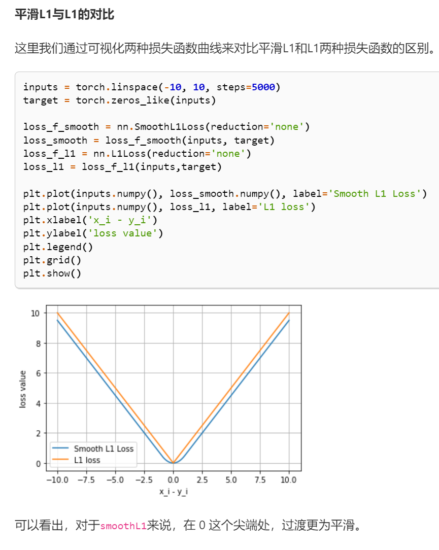
2.5.5 平滑L1 (Smooth L1)损失函数

torch.nn.SmoothL1Loss(size_average=None, reduce=None, reduction='mean', beta=1.0)

功能： L1的平滑输出，其功能是减轻离群点带来的影响

2.5.6 目标泊松分布的负对数似然损失

torch.nn.PoissonNLLLoss(log_input=True, full=False, size_average=None, eps=1e-08, reduce=None, reduction='mean')

功能： 泊松分布的负对数似然损失函数

2.5.7 KL散度

torch.nn.KLDivLoss(size_average=None, reduce=None, reduction='mean', log_target=False)

功能： 计算KL散度，也就是计算相对熵。用于连续分布的距离度量，并且对离散采用的连续输出空间分布进行回归通常很有用。

2.5.8 MarginRankingLoss

torch.nn.MarginRankingLoss(margin=0.0, size_average=None, reduce=None, reduction='mean')

功能： 计算两个向量之间的相似度，用于排序任务。该方法用于计算两组数据之间的差异。

2.5.9 多标签边界损失函数

torch.nn.MultiLabelMarginLoss(size_average=None, reduce=None, reduction='mean')

功能： 对于多标签分类问题计算损失函数。

2.5.10 二分类损失函数

torch.nn.SoftMarginLoss(size_average=None, reduce=None, reduction='mean')torch.nn.(size_average=None, reduce=None, reduction='mean')

功能： 计算二分类的 logistic 损失。

2.5.11 多分类的折页损失

torch.nn.MultiMarginLoss(p=1, margin=1.0, weight=None, size_average=None, reduce=None, reduction='mean')

功能： 计算多分类的折页损失

2.5.12 三元组损失

torch.nn.TripletMarginLoss(margin=1.0, p=2.0, eps=1e-06, swap=False, size_average=None, reduce=None, reduction='mean')

功能： 计算三元组损失。

2.5.13 HingEmbeddingLoss

torch.nn.HingeEmbeddingLoss(margin=1.0, size_average=None, reduce=None, reduction='mean')

功能： 对输出的embedding结果做Hing损失计算

2.5.14 余弦相似度

torch.nn.CosineEmbeddingLoss(margin=0.0, size_average=None, reduce=None, reduction='mean')

功能： 对两个向量做余弦相似度

2.5.15 CTC损失函数

torch.nn.CTCLoss(blank=0, reduction='mean', zero_infinity=False)

功能： 用于解决时序类数据的分类

2.6 训练和评估

这个教程里讲得就很精简了，没什么好摘抄的了，我认认真真做完笔记之后发现差不多把整页都抄下来了(。_。)

直接看教程原文吧3.7 训练和评估 — 深入浅出PyTorch (datawhalechina.github.io)

2.7 Pytorch优化器

也直接看原文吧3.9 Pytorch优化器 — 深入浅出PyTorch (datawhalechina.github.io)