python机器学习逻辑回归

数据集链接

1 Logistic回归

在该部分练习中，将建立一个逻辑回归模型，用以预测学生能否被大学录取。

假设你是大学某个部门的负责人，你要根据两次考试的结果来决定每个申请人的入学机会。目前已经有了以往申请者的历史数据，并且可以用作逻辑回归的训练集。对于每行数据，都包含对应申请者的两次考试分数和最终的录取结果。

在本次练习中，你需要建立一个分类模型，根据这两次的考试分数来预测申请者的录取结果。
要点：

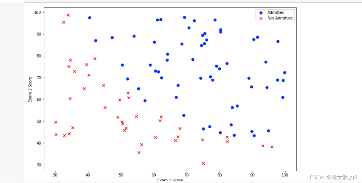
导入需要使用的python库，并将从文件ex2data1.txt中读取数据，并显示前5行
x-y轴分别为两次考试的分数
正负示例需要用不同的标记显示（不同的颜色）

import numpy as np
import pandas as pd
import matplotlib.pyplot as plt
path = '/home/jovyan/work/ex2data1.txt'
data = pd.read_csv(path, header=None, names=['Exam 1', 'Exam 2', 'Admitted'])

positive = data[data['Admitted'].isin([1])]
negative = data[data['Admitted'].isin([0])]
fig, ax = plt.subplots(figsize=(12,8))
# 正向类，绘制50个样本，c=‘b’颜色，maker=‘o’绘制的形状
ax.scatter(positive['Exam 1'], positive['Exam 2'], s=50, c='b', marker='o', label='Admitted')
ax.scatter(negative['Exam 1'], negative['Exam 2'], s=50, c='r', marker='x', label='Not Admitted')
ax.legend()# Legend 图例,获取label标签内容，如图右上角显示
ax.set_xlabel('Exam 1 Score')
ax.set_ylabel('Exam 2 Score')
plt.show()

效果

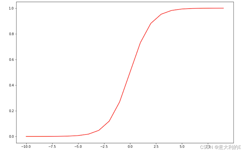
接下来，你需要编写代码实现Sigmoid函数，编写后试着测试一些值，如果x的正值较大，则函数值应接近1；如果x的负值较大，则函数值应接近0。而对于x等于0时，则函数值为0.5。

def sigmoid(z):
 return 1.0 / (1.0 + np.exp(-z))
 

nums = np.arange(-10, 10, step=1)

fig, ax = plt.subplots(figsize=(12,8))
ax.plot(nums, sigmoid(nums), 'r')
plt.show()

效果

现在，你需要编写代码实现代价函数以进行逻辑回归的成本计算，并且经过所给数据测试后，初始的成本约为0.693。

要点：

实现cost函数，参数为theta，X，y.
返回计算的成本值。
其中theta为参数，X为训练集中的特征列，y为训练集的标签列，三者均为矩阵。

def cost(theta,X,y):
    theta = np.matrix(theta)
    X = np.matrix(X)
    y = np.matrix(y)
    first = np.multiply(-y, np.log(sigmoid(X* theta.T)))
    second = np.multiply((1 - y), np.log(1 - sigmoid(X* theta.T)))
    return np.sum(first - second) / (len(X))
###请运行并测试你的代码###
def gradient(theta, X, y):
    theta = np.matrix(theta)
    X = np.matrix(X)
    y = np.matrix(y)
    
    parameters = int(theta.ravel().shape[1])
    grad = np.zeros(parameters)
    
    error = sigmoid(X * theta.T) - y
    
    for i in range(parameters):
        term = np.multiply(error, X[:,i])
        grad[i] = np.sum(term) / len(X)
    
    return grad
gradient(theta, X, y)
    

接下来，我们需要编写代码实现梯度下降用来计算我们的训练数据、标签和一些参数 𝜃
的梯度。

要点：

代码实现gradient函数，参数为theta，X，y.
返回计算的梯度值。
其中theta为参数，X为训练集中的特征列，y为训练集的标签列，三者均为矩阵。

def predict(theta, X):
    probability = sigmoid(X * theta.T)
    return [1 if x >= 0.5 else 0 for x in probability]
theta_min = np.matrix(result[0])

predictions = predict(theta_min, X)
correct = [1 if ((a == 1 and b == 1) or (a == 0 and b == 0)) else 0 for (a, b) in zip(predictions, y)]
accuracy = (sum(map(int, correct)) % len(correct))
print ('accuracy = {0}%'.format(accuracy))

2 正则化逻辑回归

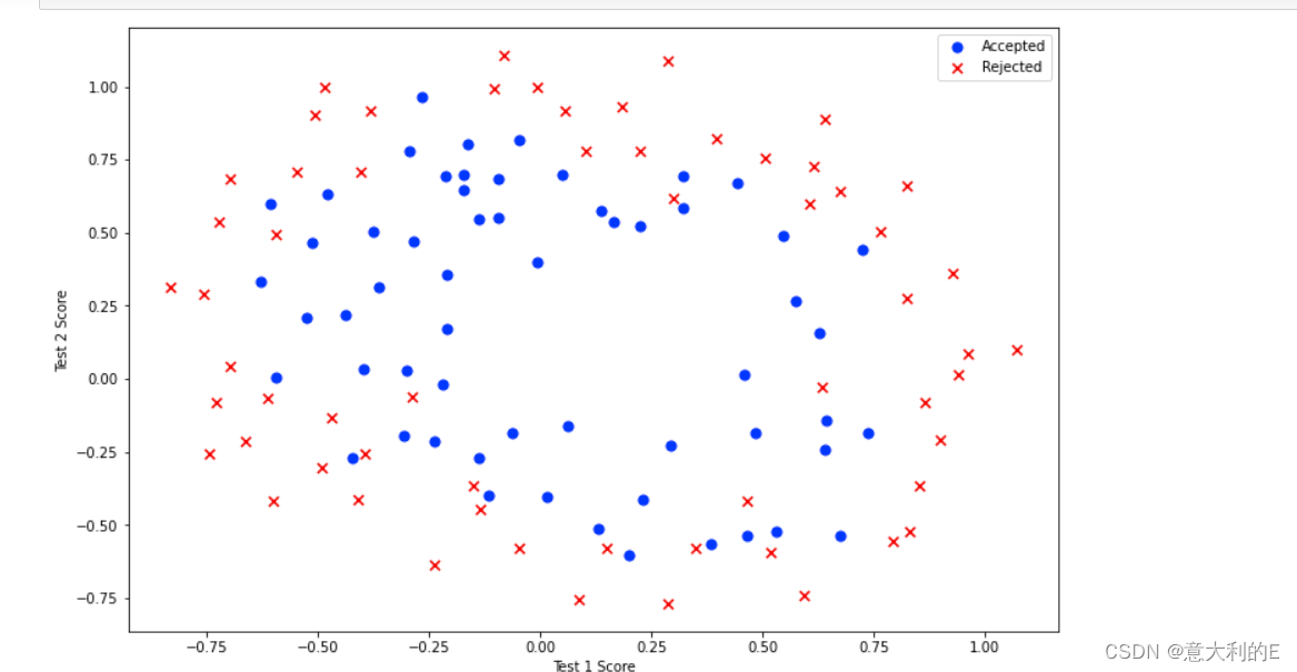
设想你是工厂的生产主管，你有一些芯片在两次测试中的测试结果。对于这两次测试，你想决定芯片是要被接受或抛弃。为了帮助你做出艰难的决定，你拥有过去芯片的测试数据集，从其中你可以构建一个逻辑回归模型。
与第一部分的练习类似，首先对数据进行可视化：

path =  '/home/jovyan/work/ex2data2.txt'
data2 = pd.read_csv(path, header=None, names=['Test 1', 'Test 2', 'Accepted'])
positive = data2[data2['Accepted'].isin([1])]
negative = data2[data2['Accepted'].isin([0])]

fig, ax = plt.subplots(figsize=(12,8))
ax.scatter(positive['Test 1'], positive['Test 2'], s=50, c='b', marker='o', label='Accepted')
ax.scatter(negative['Test 1'], negative['Test 2'], s=50, c='r', marker='x', label='Rejected')
ax.legend()
ax.set_xlabel('Test 1 Score')
ax.set_ylabel('Test 2 Score')
plt.show()

虽然特征映射允许我们构建一个更具有表现力的分类器，但它也更容易过拟合。接下来，你需要实现正则化逻辑回归用于拟合数据，并使用正则化来帮助解决过拟合问题。

# 设定映射深度
degree = 5
# 分别取两次测试的分数
x1 = data2['Test 1']
x2 = data2['Test 2']

data2.insert(3, 'Ones', 1)

# 设定计算方式进行映射
for i in range(1, degree):
    for j in range(0, i):
        data2['F' + str(i) + str(j)] = np.power(x1, i-j) * np.power(x2, j)

# 整理数据列
data2.drop('Test 1', axis=1, inplace=True)
data2.drop('Test 2', axis=1, inplace=True)

print("特征映射后具有特征维数：%d" %data2.shape[1])
data2.head()

接下来，你需要编写代码来实现计算正则化逻辑回归的代价函数和梯度，并返回计算的代价值和梯度。

正则化逻辑回归的代价函数如下：
𝐽(𝜃)=1𝑚∑𝑖=1𝑚[−𝑦(𝑖)log(ℎ𝜃(𝑥(𝑖)))−(1−𝑦(𝑖))log(1−ℎ𝜃(𝑥(𝑖)))]+𝜆2𝑚∑𝑗=1𝑛𝜃2𝑗

其中 𝜆是“学习率”参数，其值会影响函数中的正则项值。且不应该正则化参数 𝜃0。

def costReg(theta, X, y, learningRate):
    theta = np.matrix(theta)
    X = np.matrix(X)
    y = np.matrix(y)
    first = np.multiply(-y, np.log(sigmoid(X * theta.T)))
    second = np.multiply((1 - y), np.log(1 - sigmoid(X * theta.T)))
    reg = (learningRate / (2 * len(X))) * np.sum(np.power(theta[:,1:theta.shape[1]], 2))
    return np.sum(first - second) / len(X) + reg  
def gradientReg(theta, X, y, learningRate):
    theta = np.matrix(theta)
    X = np.matrix(X)
    y = np.matrix(y)
    
    parameters = int(theta.ravel().shape[1])
    grad = np.zeros(parameters)
    
    error = sigmoid(X * theta.T) - y
    
    for i in range(parameters):
        term = np.multiply(error, X[:,i])
        
        if (i == 0):
            grad[i] = np.sum(term) / len(X)
        else:
            grad[i] = (np.sum(term) / len(X)) + ((learningRate / len(X)) * theta[:,i])
    
    return grad
# 从数据集中取得对应的特征列和标签列
cols = data2.shape[1]
X2 = data2.iloc[:,1:cols]
y2 = data2.iloc[:,0:1]

# 转换为Numpy数组并初始化theta为零矩阵
X2 = np.array(X2.values)
y2 = np.array(y2.values)
theta2 = np.zeros(11)

# 设置初始学习率为1，后续可以修改
learningRate = 1    
    

接下来，使用初始化的变量值来测试你实现的代价函数和梯度函数。使用和第一部分相同的优化函数来计算优化后的结果。

costReg(theta2, X2, y2, learningRate)
gradientReg(theta2, X2, y2, learningRate)
result2 = opt.fmin_tnc(func=costReg, x0=theta2, fprime=gradientReg, args=(X2, y2, learningRate))

最后，我们可以使用第1部分中的预测函数来查看我们的方案在训练数据上的准确度。

theta_min = np.matrix(result2[0])
predictions = predict(theta_min, X2)
correct = [1 if ((a == 1 and b == 1) or (a == 0 and b == 0)) else 0 for (a, b) in zip(predictions, y2)]
accuracy = (sum(map(int, correct)) % len(correct))
print ('accuracy = {0}%'.format(accuracy))