


Analyzing RNA-seq data with DESeq2
A basic task in the analysis of count data from RNA-seq is the detection of differentially expressed genes. The count data are presented as a table which reports, for each sample, the number of sequence fragments that have been assigned to each gene. Analogous data also arise for other assay types, including comparative ChIP-Seq, HiC, shRNA screening, and mass spectrometry. An important analysis question is the quantification and statistical inference of systematic changes between conditions, as compared to within-condition variability. The package DESeq2 provides methods to test for differential expression by use of negative binomial generalized linear models; the estimates of dispersion and logarithmic fold changes incorporate data-driven prior distributions. This vignette explains the use of the package and demonstrates typical workflows. An RNA-seq workflow on the Bioconductor website covers similar material to this vignette but at a slower pace, including the generation of count matrices from FASTQ files. DESeq2 package version: 1.36.0
DESeq2 Algorithm DESeq2 (v1.0)
DESeq2 is a popular algorithm for analyzing RNA-seq data [2], which estimates the variance-mean depending in high-throughput count data, and determines differential expression based on a negative binomial distribution [3]. DESeq2 improves upon the previously published DESeq algorithm, by improving stability and interpretability of expression estimates.
The GenePattern DESeq2 module takes RNA-Seq raw count data as an input, in the GCT file format. These raw count values can be generated by HTSeq-Count [4], which determines un-normalized count values from aligned sequencing reads and a list of genomic features (e.g. genes or exons). The HTSeq-Count tool is not currently available on GenePattern. If you have data from HTSeq-counts, the GenePattern MergeHTSeqCountx module will merge multiple samples together into one GCT file, which can then be passed to DESeq2. Note that DESeq2 will not accept normalized RPKM or FPKM values, only raw count data.
In addition to the raw count data in GCT format, the DESeq2 module requires a class file in the CLS format, which categorizes samples based on, e.g. phenotype, treatment, cell type, etc. DESeq2 completes differential expression analysis based on the annoted classes in this file. DESeq2 also optionally accepts a confounding variable class file. This will be included in the DESeq2 design formula allowign DESeq2 to comupte the differntial expression of the classes in the first CLS controlling for the effect of the variables in the confounding variable CLS.
Note that, in this first release of DESeq2, two-factor analysis has not been enabled. That feature will be enabled in a future release.
Parameters
| Name | Description |
|---|---|
| input file * | A GCT file containing raw RNA-Seq counts, such as is produced by MergeHTSeqCounts |
| cls file * | A categorical CLS file specifying the phenotype classes for the samples in the GCT file. This should contain exactly two classes with the control specified first. |
| confounding variable cls file | A categorical CLS file specifying an additional confounding variable, mapped to the input file samples. |
| output file base * | The base name of the output file(s). File extensions will be added automatically. |
| qc plot format * | Choose a file format for the QC plots (or skip them completely) |
| fdr threshold * | FDR threshold to use in filtering before creating the reports of top up-regulated and down-regulated genes |
| top N count * | Max gene count to use when creating the reports of top up-regulated and down-regulated genes |
| random seed * | Seed to use for randomization |
* - required
Input Files
- input file DESeq2/gpunit/Input at develop · genepattern/DESeq2 · GitHub
The GenePattern DESeq2 module takes RNA-Seq raw count data as an input, in the GCT file format. These raw count values can be generated by HTSeq-Count, which determines un-normalized count values from aligned sequencing reads and a list of genomic features (e.g. genes or exons). The HTSeq-Count tool is not yet available on GenePattern. If you have .count data from HTSeq-count, run outside of GenePattern, the GenePattern MergeHTSeqCounts module will merge multiple samples together into one GCT file, which can then be passed to DESeq2. Note that DESeq2 will not accept normalized RPKM or FPKM values, only raw count data. - cls file
In addition to the raw count data in GCT format, the DESeq2 module requires a class file in the CLS format, which categorizes samples based on, e.g. phenotype, treatment, cell type, etc. - confounding variable cls file
In addition, DESeq2 accepts a confounding class file, which re-categorizes samples according to a secondary class.
- Standard workflow
- Data transformations and visualization
- Variations to the standard workflow
- Wald test individual steps
- Contrasts
- Interactions
- Time-series experiments
- Likelihood ratio test
- Extended section on shrinkage estimators
- Recommendations for single-cell analysis
- Approach to count outliers
- Dispersion plot and fitting alternatives
- Independent filtering of results
- Tests of log2 fold change above or below a threshold
- Access to all calculated values
- Sample-/gene-dependent normalization factors
- “Model matrix not full rank”
- Theory behind DESeq2
- Frequently asked questions
- How can I get support for DESeq2?
- Why are some p values set to NA?
- How can I get unfiltered DESeq2 results?
- How do I use VST or rlog data for differential testing?
- Why after VST are there still batches in the PCA plot?
- Do normalized counts correct for variables in the design?
- Can I use DESeq2 to analyze paired samples?
- If I have multiple groups, should I run all together or split into pairs of groups?
- Can I run DESeq2 to contrast the levels of many groups?
- Can I use DESeq2 to analyze a dataset without replicates?
- How can I include a continuous covariate in the design formula?
- I ran a likelihood ratio test, but results() only gives me one comparison.
- What are the exact steps performed by DESeq()?
- Is there an official Galaxy tool for DESeq2?
- I want to benchmark DESeq2 comparing to other DE tools.
- I have trouble installing DESeq2 on Ubuntu/Linux…
- Session info
- References
Quick start
Here we show the most basic steps for a differential expression analysis. There are a variety of steps upstream of DESeq2 that result in the generation of counts or estimated counts for each sample, which we will discuss in the sections below. This code chunk assumes that you have a count matrix called cts and a table of sample information called coldata. The design indicates how to model the samples, here, that we want to measure the effect of the condition, controlling for batch differences. The two factor variables batch and condition should be columns of coldata.
dds <- DESeqDataSetFromMatrix(countData = cts,
                              colData = coldata,
                              design= ~ batch + condition)
dds <- DESeq(dds)
resultsNames(dds) # lists the coefficients
res <- results(dds, name="condition_trt_vs_untrt")
# or to shrink log fold changes association with condition:
res <- lfcShrink(dds, coef="condition_trt_vs_untrt", type="apeglm")coldata## condition type
## treated1fb treated single-read
## treated2fb treated paired-end
## treated3fb treated paired-end
## untreated1fb untreated single-read
## untreated2fb untreated single-read
## untreated3fb untreated paired-end
## untreated4fb untreated paired-endNote that these are not in the same order with respect to samples!
It is absolutely critical that the columns of the count matrix and the rows of the column data (information about samples) are in the same order. DESeq2 will not make guesses as to which column of the count matrix belongs to which row of the column data, these must be provided to DESeq2 already in consistent order.
As they are not in the correct order as given, we need to re-arrange one or the other so that they are consistent in terms of sample order (if we do not, later functions would produce an error). We additionally need to chop off the "fb" of the row names of coldata, so the naming is consistent.
rownames(coldata) <- sub("fb", "", rownames(coldata))
all(rownames(coldata) %in% colnames(cts))
The following starting functions will be explained below:
- If you have performed transcript quantification (with Salmon, kallisto, RSEM, etc.) you could import the data with tximport, which produces a list, and then you can use
DESeqDataSetFromTximport(). - If you imported quantification data with tximeta, which produces a SummarizedExperiment with additional metadata, you can then use
DESeqDataSet(). - If you have htseq-count files, you can use
DESeqDataSetFromHTSeq().
How to get help for DESeq2
Any and all DESeq2 questions should be posted to the Bioconductor support site, which serves as a searchable knowledge base of questions and answers:
https://support.bioconductor.org
Posting a question and tagging with “DESeq2” will automatically send an alert to the package authors to respond on the support site. See the first question in the list of Frequently Asked Questions (FAQ) for information about how to construct an informative post.
You should not email your question to the package authors, as we will just reply that the question should be posted to the Bioconductor support site.
Input data 输入数据格式要求 输入数据必须为rawdata 未normalized数据
Why un-normalized counts?
As input, the DESeq2 package expects count data as obtained, e.g., from RNA-seq or another high-throughput sequencing experiment, in the form of a matrix of integer values. The value in the i-th row and the j-th column of the matrix tells how many reads can be assigned to gene i in sample j. Analogously, for other types of assays, the rows of the matrix might correspond e.g. to binding regions (with ChIP-Seq) or peptide sequences (with quantitative mass spectrometry). We will list method for obtaining count matrices in sections below.
The values in the matrix should be un-normalized counts or estimated counts of sequencing reads (for single-end RNA-seq) or fragments (for paired-end RNA-seq). The RNA-seq workflow describes multiple techniques for preparing such count matrices. It is important to provide count matrices as input for DESeq2’s statistical model (Love, Huber, and Anders 2014) to hold, as only the count values allow assessing the measurement precision correctly. The DESeq2 model internally corrects for library size, so transformed or normalized values such as counts scaled by library size should not be used as input.
The DESeqDataSet deseq2所用到的中间数据结构叫做dds
The object class used by the DESeq2 package to store the read counts and the intermediate estimated quantities during statistical analysis is the DESeqDataSet, which will usually be represented in the code here as an object dds.
A technical detail is that the DESeqDataSet class extends the RangedSummarizedExperiment class of the SummarizedExperiment package. The “Ranged” part refers to the fact that the rows of the assay data (here, the counts) can be associated with genomic ranges (the exons of genes). This association facilitates downstream exploration of results, making use of other Bioconductor packages’ range-based functionality (e.g. find the closest ChIP-seq peaks to the differentially expressed genes).
A DESeqDataSet object must have an associated design formula. The design formula expresses the variables which will be used in modeling. The formula should be a tilde (~) followed by the variables with plus signs between them (it will be coerced into an formula if it is not already). The design can be changed later, however then all differential analysis steps should be repeated, as the design formula is used to estimate the dispersions and to estimate the log2 fold changes of the model.
Note: In order to benefit from the default settings of the package, you should put the variable of interest at the end of the formula and make sure the control level is the first level.
We will now show 4 ways of constructing a DESeqDataSet, depending on what pipeline was used upstream of DESeq2 to generated counts or estimated counts:
- From transcript abundance files and tximport
- From a count matrix
- From htseq-count files
- From a SummarizedExperiment object
SummarizedExperiment input
If one has already created or obtained a SummarizedExperiment, it can be easily input into DESeq2 as follows. First we load the package containing the airway dataset.
library("airway")
data("airway")
se <- airway
The constructor function below shows the generation of a DESeqDataSet from a RangedSummarizedExperiment se.
library("DESeq2")
ddsSE <- DESeqDataSet(se, design = ~ cell + dex)
ddsSE
## class: DESeqDataSet
## dim: 64102 8
## metadata(2): '' version
## assays(1): counts
## rownames(64102): ENSG00000000003 ENSG00000000005 ... LRG_98 LRG_99
## rowData names(0):
## colnames(8): SRR1039508 SRR1039509 ... SRR1039520 SRR1039521
## colData names(9): SampleName cell ... Sample BioSamplePre-filtering
While it is not necessary to pre-filter low count genes before running the DESeq2 functions, there are two reasons which make pre-filtering useful: by removing rows in which there are very few reads, we reduce the memory size of the dds data object, and we increase the speed of the transformation and testing functions within DESeq2. Here we perform a minimal pre-filtering to keep only rows that have at least 10 reads total. Note that more strict filtering to increase power is automatically applied via independent filtering on the mean of normalized counts within the results function.
keep <- rowSums(counts(dds)) >= 10
dds <- dds[keep,]
Note on factor levels 谁是control组 谁是被比较组别
By default, R will choose a reference level for factors based on alphabetical order. Then, if you never tell the DESeq2 functions which level you want to compare against (e.g. which level represents the control group), the comparisons will be based on the alphabetical order of the levels. There are two solutions: you can either explicitly tell results which comparison to make using the contrast argument (this will be shown later), or you can explicitly set the factors levels. In order to see the change of reference levels reflected in the results names, you need to either run DESeq or nbinomWaldTest/nbinomLRT after the re-leveling operation. Setting the factor levels can be done in two ways, either using factor:
dds$condition <- factor(dds$condition, levels = c("untreated","treated"))…or using relevel, just specifying the reference level:
dds$condition <- relevel(dds$condition, ref = "untreated")If you need to subset the columns of a DESeqDataSet, i.e., when removing certain samples from the analysis, it is possible that all the samples for one or more levels of a variable in the design formula would be removed. In this case, the droplevels function can be used to remove those levels which do not have samples in the current DESeqDataSet:
dds$condition <- droplevels(dds$condition)Collapsing technical replicates 技术重复 不是生物学 重复怎么办!!
DESeq2 provides a function collapseReplicates which can assist in combining the counts from technical replicates into single columns of the count matrix. The term technical replicate implies multiple sequencing runs of the same library. You should not collapse biological replicates using this function. See the manual page for an example of the use of collapseReplicates.
About the pasilla dataset
We continue with the pasilla data constructed from the count matrix method above. This data set is from an experiment on Drosophila melanogaster cell cultures and investigated the effect of RNAi knock-down of the splicing factor pasilla (Brooks et al. 2011). The detailed transcript of the production of the pasilla data is provided in the vignette of the data package pasilla.
Differential expression analysis
The standard differential expression analysis steps are wrapped into a single function, DESeq. The estimation steps performed by this function are described below, in the manual page for ?DESeq and in the Methods section of the DESeq2 publication (Love, Huber, and Anders 2014).
Results tables are generated using the function results, which extracts a results table with log2 fold changes, p values and adjusted p values. With no additional arguments to results, the log2 fold change and Wald test p value will be for the last variable in the design formula, and if this is a factor, the comparison will be the last level of this variable over the reference level (see previous note on factor levels). However, the order of the variables of the design do not matter so long as the user specifies the comparison to build a results table for, using the name or contrast arguments of results.
Details about the comparison are printed to the console, directly above the results table. The text, condition treated vs untreated, tells you that the estimates are of the logarithmic fold change log2(treated/untreated).
dds <- DESeq(dds)
res <- results(dds)
re
## log2 fold change (MLE): condition treated vs untreated
## Wald test p-value: condition treated vs untreated
## DataFrame with 9921 rows and 6 columns
## baseMean log2FoldChange lfcSE stat pvalue padj
## <numeric> <numeric> <numeric> <numeric> <numeric> <numeric>
## FBgn0000008 95.14429 0.00227644 0.223729 0.010175 0.9918817 0.997211
## FBgn0000014 1.05652 -0.49512039 2.143186 -0.231021 0.8172987 NA
## FBgn0000017 4352.55357 -0.23991894 0.126337 -1.899041 0.0575591 0.288002
## FBgn0000018 418.61048 -0.10467391 0.148489 -0.704927 0.4808558 0.826834
## FBgn0000024 6.40620 0.21084779 0.689588 0.305759 0.7597879 0.943501
## ... ... ... ... ... ... ...
## FBgn0261570 3208.38861 0.2955329 0.127350 2.3206264 0.020307 0.144240
## FBgn0261572 6.19719 -0.9588230 0.775315 -1.2366888 0.216203 0.607848
## FBgn0261573 2240.97951 0.0127194 0.113300 0.1122634 0.910615 0.982657
## FBgn0261574 4857.68037 0.0153924 0.192567 0.0799327 0.936291 0.988179
## FBgn0261575 10.68252 0.1635705 0.930911 0.1757102 0.860522 0.967928Note that we could have specified the coefficient or contrast we want to build a results table for, using either of the following equivalent commands:
res <- results(dds, name="condition_treated_vs_untreated")
res <- results(dds, contrast=c("condition","treated","untreated"))
One exception to the equivalence of these two commands, is that, using contrast will additionally set to 0 the estimated LFC in a comparison of two groups, where all of the counts in the two groups are equal to 0 (while other groups have positive counts). As this may be a desired feature to have the LFC in these cases set to 0, one can use contrast to build these results tables. More information about extracting specific coefficients from a fitted DESeqDataSet object can be found in the help page ?results. The use of the contrast argument is also further discussed below.
Log fold change shrinkage for visualization and ranking 热图火山图很丑怎么办? 进行收缩!! Analyzing RNA-seq data with DESeq2
数据收缩:lfcShrink:https://www.jianshu.com/p/8aa995149744
shrink the log2 foldchange,不会改变显著差异的基因总数,
Shrinkage of effect size (LFC estimates) is useful for visualization and ranking of genes. To shrink the LFC, we pass the dds object to the function lfcShrink. Below we specify to use the apeglm method for effect size shrinkage (Zhu, Ibrahim, and Love 2018), which improves on the previous estimator.
We provide the dds object and the name or number of the coefficient we want to shrink, where the number refers to the order of the coefficient as it appears in resultsNames(dds).
resultsNames(dds)## [1] "Intercept" "condition_treated_vs_untreated"resLFC <- lfcShrink(dds, coef="condition_treated_vs_untreated", type="apeglm")
resLFC## log2 fold change (MAP): condition treated vs untreated
## Wald test p-value: condition treated vs untreated
## DataFrame with 9921 rows and 5 columns
## baseMean log2FoldChange lfcSE pvalue padj
## <numeric> <numeric> <numeric> <numeric> <numeric>
## FBgn0000008 95.14429 0.00119920 0.151897 0.9918817 0.997211
## FBgn0000014 1.05652 -0.00473412 0.205468 0.8172987 NA
## FBgn0000017 4352.55357 -0.18989990 0.120377 0.0575591 0.288002
## FBgn0000018 418.61048 -0.06995753 0.123901 0.4808558 0.826834
## FBgn0000024 6.40620 0.01752715 0.198633 0.7597879 0.943501
## ... ... ... ... ... ...
## FBgn0261570 3208.38861 0.24110290 0.1244469 0.020307 0.144240
## FBgn0261572 6.19719 -0.06576173 0.2141351 0.216203 0.607848
## FBgn0261573 2240.97951 0.01000619 0.0993764 0.910615 0.982657
## FBgn0261574 4857.68037 0.00843552 0.1408267 0.936291 0.988179
## FBgn0261575 10.68252 0.00809101 0.2014704 0.860522 0.967928Shrinkage estimation is discussed more in a later section.
Speed-up and parallelization thoughts deseq2运行速度太慢怎么办!
The above steps should take less than 30 seconds for most analyses. For experiments with complex designs and many samples (e.g. dozens of coefficients, ~100s of samples), one may want to have faster computation than provided by the default run of DESeq. We have two recommendations:
-
By using the argument
fitType="glmGamPoi", one can leverage the faster NB GLM engine written by Constantin Ahlmann-Eltze. Note that glmGamPoi’s interface in DESeq2 requires use oftest="LRT"and specification of areduceddesign. -
One can take advantage of parallelized computation. Parallelizing
DESeq,results, andlfcShrinkcan be easily accomplished by loading the BiocParallel package, and then setting the following arguments:parallel=TRUEandBPPARAM=MulticoreParam(4), for example, splitting the job over 4 cores. However, some words of advice on parallelization: first, it is recommend to filter genes where all samples have low counts, to avoid sending data unnecessarily to child processes, when those genes have low power and will be independently filtered anyway; secondly, there is often diminishing returns for adding more cores due to overhead of sending data to child processes, therefore I recommend first starting with small number of additional cores. Note that obtainingresultsfor coefficients or contrasts listed inresultsNames(dds)is fast and will not need parallelization. As an alternative toBPPARAM, one canregistercores at the beginning of an analysis, and then just specifyparallel=TRUEto the functions when called.
library("BiocParallel")
register(MulticoreParam(4))
p-values and adjusted p-values 对结果进行过滤删选 cutoff
We can order our results table by the smallest p value:
resOrdered <- res[order(res$pvalue),]We can summarize some basic tallies using the summary function.
summary(res)##
## out of 9921 with nonzero total read count
## adjusted p-value < 0.1
## LFC > 0 (up) : 518, 5.2%
## LFC < 0 (down) : 536, 5.4%
## outliers [1] : 1, 0.01%
## low counts [2] : 1539, 16%
## (mean count < 6)
## [1] see 'cooksCutoff' argument of ?results
## [2] see 'independentFiltering' argument of ?resultsHow many adjusted p-values were less than 0.1?
sum(res$padj < 0.1, na.rm=TRUE)## [1] 1054The results function contains a number of arguments to customize the results table which is generated. You can read about these arguments by looking up ?results. Note that the results function automatically performs independent filtering based on the mean of normalized counts for each gene, optimizing the number of genes which will have an adjusted p value below a given FDR cutoff, alpha. Independent filtering is further discussed below. By default the argument alpha is set to 0.1. If the adjusted p value cutoff will be a value other than 0.1, alpha should be set to that value:
res05 <- results(dds, alpha=0.05)
summary(res05)
##
## out of 9921 with nonzero total read count
## adjusted p-value < 0.05
## LFC > 0 (up) : 407, 4.1%
## LFC < 0 (down) : 431, 4.3%
## outliers [1] : 1, 0.01%
## low counts [2] : 1347, 14%
## (mean count < 5)
## [1] see 'cooksCutoff' argument of ?results
## [2] see 'independentFiltering' argument of ?resultssum(res05$padj < 0.05, na.rm=TRUE)## [1] 838Independent hypothesis weighting 可以忽略此步骤 专为高级用户
A generalization of the idea of p value filtering is to weight hypotheses to optimize power. A Bioconductor package, IHW, is available that implements the method of Independent Hypothesis Weighting (Ignatiadis et al. 2016). Here we show the use of IHW for p value adjustment of DESeq2 results. For more details, please see the vignette of the IHW package. The IHW result object is stored in the metadata.
Note: If the results of independent hypothesis weighting are used in published research, please cite:
Ignatiadis, N., Klaus, B., Zaugg, J.B., Huber, W. (2016) Data-driven hypothesis weighting increases detection power in genome-scale multiple testing. Nature Methods, 13:7. 10.1038/nmeth.3885
# (unevaluated code chunk)
library("IHW")
resIHW <- results(dds, filterFun=ihw)
summary(resIHW)
sum(resIHW$padj < 0.1, na.rm=TRUE)
metadata(resIHW)$ihwResult
For advanced users, note that all the values calculated by the DESeq2 package are stored in the DESeqDataSet object or the DESeqResults object, and access to these values is discussed below.
Exploring and exporting results
MA-plot
In DESeq2, the function plotMA shows the log2 fold changes attributable to a given variable over the mean of normalized counts for all the samples in the DESeqDataSet. Points will be colored red if the adjusted p value is less than 0.1. Points which fall out of the window are plotted as open triangles pointing either up or down.
plotMA(res, ylim=c(-2,2))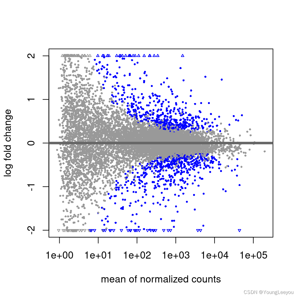
It is more useful visualize the MA-plot for the shrunken log2 fold changes, which remove the noise associated with log2 fold changes from low count genes without requiring arbitrary filtering thresholds.
plotMA(resLFC, ylim=c(-2,2))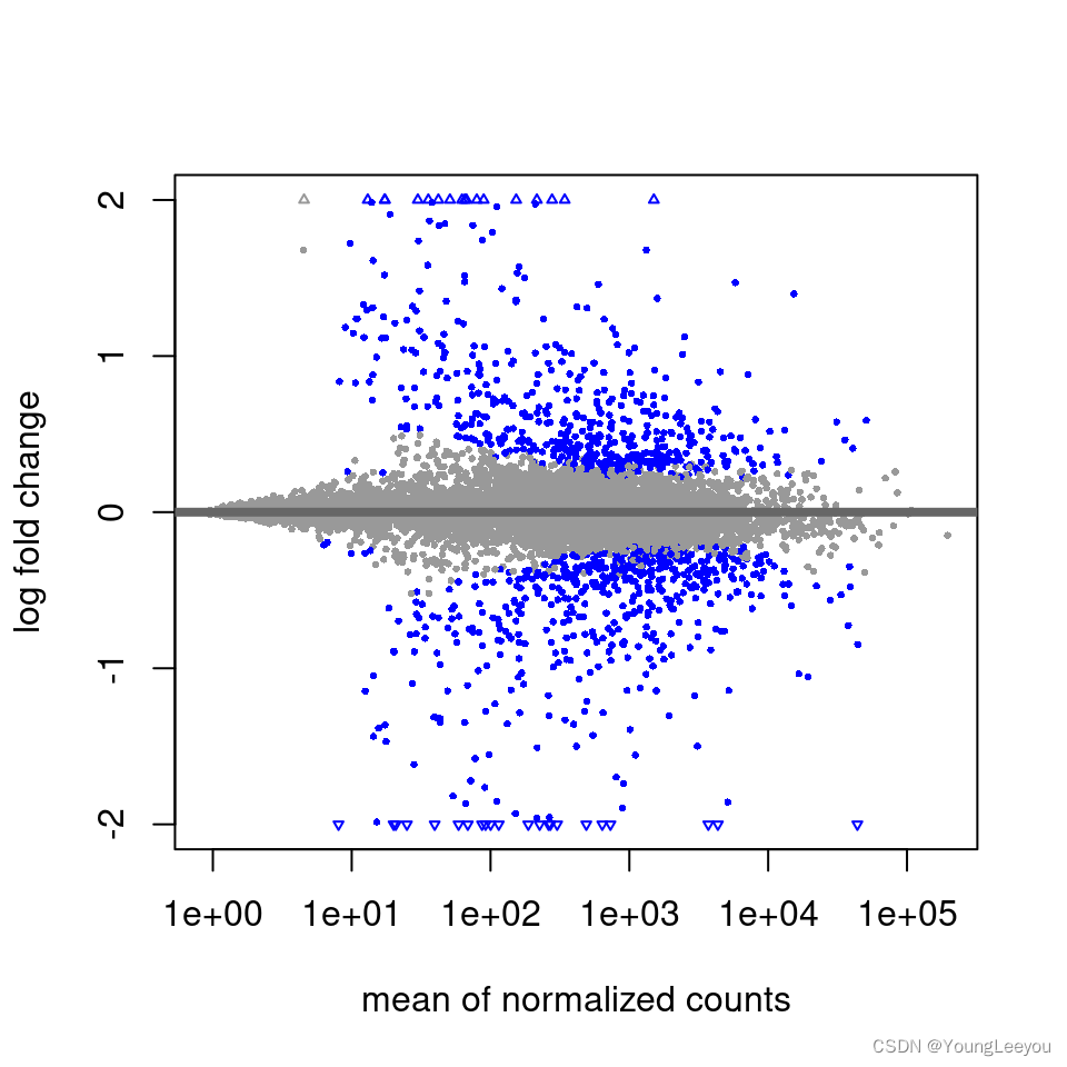
After calling plotMA, one can use the function identify to interactively detect the row number of individual genes by clicking on the plot. One can then recover the gene identifiers by saving the resulting indices:
idx <- identify(res$baseMean, res$log2FoldChange)
rownames(res)[idx]
Plot counts 如何画单个基因的表达
It can also be useful to examine the counts of reads for a single gene across the groups. A simple function for making this plot is plotCounts, which normalizes counts by the estimated size factors (or normalization factors if these were used) and adds a pseudocount of 1/2 to allow for log scale plotting. The counts are grouped by the variables in intgroup, where more than one variable can be specified. Here we specify the gene which had the smallest p value from the results table created above. You can select the gene to plot by rowname or by numeric index.
plotCounts(dds, gene=which.min(res$padj), intgroup="condition")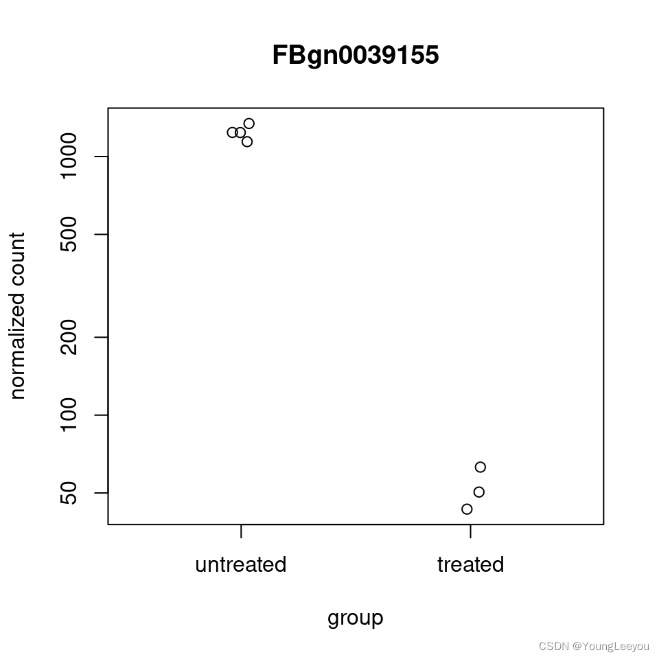
For customized plotting, an argument returnData specifies that the function should only return a data.frame for plotting with ggplot.
d <- plotCounts(dds, gene=which.min(res$padj), intgroup="condition",
                returnData=TRUE)
library("ggplot2")
ggplot(d, aes(x=condition, y=count)) +
  geom_point(position=position_jitter(w=0.1,h=0)) +
  scale_y_log10(breaks=c(25,100,400))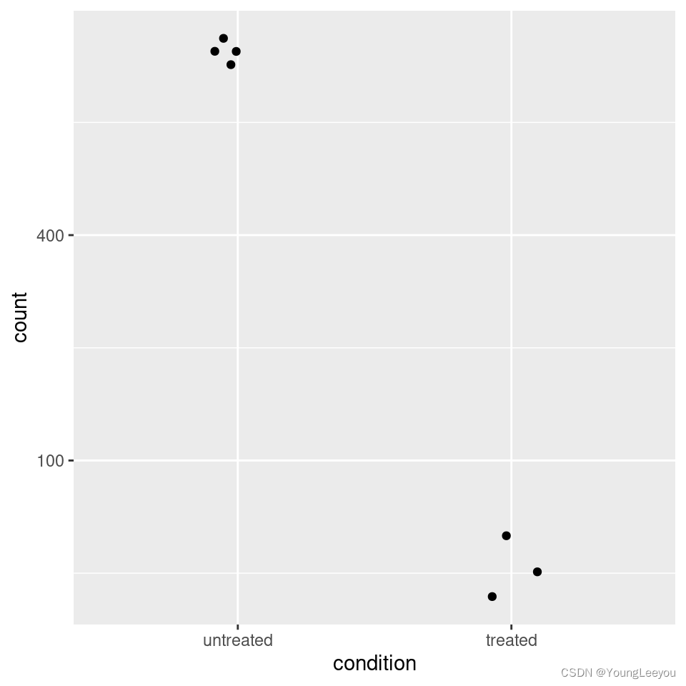
More information on results columns
Information about which variables and tests were used can be found by calling the function mcols on the results object.
mcols(res)$description## [1] "mean of normalized counts for all samples"
## [2] "log2 fold change (MLE): condition treated vs untreated"
## [3] "standard error: condition treated vs untreated"
## [4] "Wald statistic: condition treated vs untreated"
## [5] "Wald test p-value: condition treated vs untreated"
## [6] "BH adjusted p-values"For a particular gene, a log2 fold change of -1 for condition treated vs untreated means that the treatment induces a multiplicative change in observed gene expression level of 2−1=0.52−1=0.5 compared to the untreated condition. If the variable of interest is continuous-valued, then the reported log2 fold change is per unit of change of that variable.
Note on p-values set to NA: some values in the results table can be set to NA for one of the following reasons: NA值怎么办
- If within a row, all samples have zero counts, the
baseMeancolumn will be zero, and the log2 fold change estimates, p value and adjusted p value will all be set toNA. - If a row contains a sample with an extreme count outlier then the p value and adjusted p value will be set to
NA. These outlier counts are detected by Cook’s distance. Customization of this outlier filtering and description of functionality for replacement of outlier counts and refitting is described below - If a row is filtered by automatic independent filtering, for having a low mean normalized count, then only the adjusted p value will be set to
NA. Description and customization of independent filtering is described below
Rich visualization and reporting of results 导出结果 各种方式对结果进行可视化 各种花里胡哨的可视化结果 html格式 公司格式 结果报告结果 report html
ReportingTools An HTML report of the results with plots and sortable/filterable columns can be generated using the ReportingTools package on a DESeqDataSet that has been processed by the DESeq function. For a code example, see the RNA-seq differential expression vignette at the ReportingTools page, or the manual page for the publish method for the DESeqDataSet class.
regionReport An HTML and PDF summary of the results with plots can also be generated using the regionReport package. The DESeq2Report function should be run on a DESeqDataSet that has been processed by the DESeq function. For more details see the manual page for DESeq2Report and an example vignette in the regionReport package.
Glimma Interactive visualization of DESeq2 output, including MA-plots (also called MD-plot) can be generated using the Glimma package. See the manual page for glMDPlot.DESeqResults.
pcaExplorer Interactive visualization of DESeq2 output, including PCA plots, boxplots of counts and other useful summaries can be generated using the pcaExplorer package. See the Launching the application section of the package vignette.
iSEE Provides functions for creating an interactive Shiny-based graphical user interface for exploring data stored in SummarizedExperiment objects, including row- and column-level metadata. Particular attention is given to single-cell data in a SingleCellExperiment object with visualization of dimensionality reduction results. iSEE is on Bioconductor. An example wrapper function for converting a DESeqDataSet to a SingleCellExperiment object for use with iSEE can be found at the following gist, written by Federico Marini:
DEvis DEvis is a powerful, integrated solution for the analysis of differential expression data. This package includes an array of tools for manipulating and aggregating data, as well as a wide range of customizable visualizations, and project management functionality that simplify RNA-Seq analysis and provide a variety of ways of exploring and analyzing data. DEvis can be found on CRAN and GitHub.
Exporting results to CSV files
A plain-text file of the results can be exported using the base R functions write.csv or write.delim. We suggest using a descriptive file name indicating the variable and levels which were tested.
write.csv(as.data.frame(resOrdered),
          file="condition_treated_results.csv")
Exporting only the results which pass an adjusted p value threshold can be accomplished with the subset function, followed by the write.csv function.
resSig <- subset(resOrdered, padj < 0.1)
resSig
## log2 fold change (MLE): condition treated vs untreated
## Wald test p-value: condition treated vs untreated
## DataFrame with 1054 rows and 6 columns
## baseMean log2FoldChange lfcSE stat pvalue
## <numeric> <numeric> <numeric> <numeric> <numeric>
## FBgn0039155 730.568 -4.61874 0.1691240 -27.3098 3.24447e-164
## FBgn0025111 1501.448 2.89995 0.1273576 22.7701 9.07164e-115
## FBgn0029167 3706.024 -2.19691 0.0979154 -22.4368 1.72030e-111
## FBgn0003360 4342.832 -3.17954 0.1435677 -22.1466 1.12417e-108
## FBgn0035085 638.219 -2.56024 0.1378126 -18.5777 4.86845e-77
## ... ... ... ... ... ...
## FBgn0037073 973.1016 -0.252146 0.1009872 -2.49681 0.0125316
## FBgn0029976 2312.5885 -0.221127 0.0885764 -2.49645 0.0125443
## FBgn0030938 24.8064 0.957645 0.3836454 2.49617 0.0125542
## FBgn0039260 1088.2766 -0.259253 0.1038739 -2.49585 0.0125656
## FBgn0034753 7775.2711 0.393515 0.1576749 2.49574 0.0125696
## padj
## <numeric>
## FBgn0039155 2.71919e-160
## FBgn0025111 3.80147e-111
## FBgn0029167 4.80595e-108
## FBgn0003360 2.35542e-105
## FBgn0035085 8.16049e-74
## ... ...
## FBgn0037073 0.0999489
## FBgn0029976 0.0999489
## FBgn0030938 0.0999489
## FBgn0039260 0.0999489
## FBgn0034753 0.0999489Multi-factor designs 多个因素可能影响差异分析的结果怎么办
根据性别 是否抽烟 如何调整差异分析p值 deseq2 根据性别如何调整差异分析p值 多因素差异分析deseq2
To identify differences in protein-coding gene expression profiles, we compared the transcriptional signatures between CHP and controls, and between IPF and controls, adjusting for sex, race, age, plate, institution, and smoking history using DESeq2. In surgical lung biopsy specimens, we identified 907 upregulated and 1,077 downregulated genes as differentially expressed between subjects with CHP and control subjects, whereas 1,077 upregulated and 480 downregulated genes were differentially expressed between subjects with IPF and control subjects at a false discovery rate–adjusted P value,0.05 and absolute log2 fold change.1 (Figures 1A and 1B).Chronic Hypersensitivity Pneumonitis, an Interstitial Lung Disease with Distinct Molecular Signatures
Experiments with more than one factor influencing the counts can be analyzed using design formula that include the additional variables. In fact, DESeq2 can analyze any possible experimental design that can be expressed with fixed effects terms (multiple factors, designs with interactions, designs with continuous variables, splines, and so on are all possible).
By adding variables to the design, one can control for additional variation in the counts. For example, if the condition samples are balanced across experimental batches, by including the batch factor to the design, one can increase the sensitivity for finding differences due to condition. There are multiple ways to analyze experiments when the additional variables are of interest and not just controlling factors (see section on interactions).
The data in the pasilla package have a condition of interest (the column condition), as well as information on the type of sequencing which was performed (the column type), as we can see below:
colData(dds)## DataFrame with 7 rows and 3 columns
## condition type sizeFactor
## <factor> <factor> <numeric>
## treated1 treated single-read 1.635501
## treated2 treated paired-end 0.761216
## treated3 treated paired-end 0.832660
## untreated1 untreated single-read 1.138338
## untreated2 untreated single-read 1.793541
## untreated3 untreated paired-end 0.649483
## untreated4 untreated paired-end 0.751600We create a copy of the DESeqDataSet, so that we can rerun the analysis using a multi-factor design.
ddsMF <- ddsWe change the levels of type so it only contains letters (numbers, underscore and period are also allowed in design factor levels). Be careful when changing level names to use the same order as the current levels. 给type重命名 更符合视觉效果
levels(ddsMF$type)## [1] "paired-end" "single-read"levels(ddsMF$type) <- sub("-.*", "", levels(ddsMF$type))
levels(ddsMF$type)## [1] "paired" "single"We can account for the different types of sequencing, and get a clearer picture of the differences attributable to the treatment. As condition is the variable of interest, we put it at the end of the formula. Thus the results function will by default pull the condition results unless contrast or name arguments are specified. 多因素差异分析deseq2
Then we can re-run DESeq:
design(ddsMF) <- formula(~ type + condition)
ddsMF <- DESeq(ddsMF)
Again, we access the results using the results function.
resMF <- results(ddsMF)
head(resMF)
## log2 fold change (MLE): condition treated vs untreated
## Wald test p-value: condition treated vs untreated
## DataFrame with 6 rows and 6 columns
## baseMean log2FoldChange lfcSE stat pvalue padj
## <numeric> <numeric> <numeric> <numeric> <numeric> <numeric>
## FBgn0000008 95.14429 -0.0405571 0.220040 -0.1843169 0.8537648 0.949444
## FBgn0000014 1.05652 -0.0835022 2.075676 -0.0402289 0.9679106 NA
## FBgn0000017 4352.55357 -0.2560570 0.112230 -2.2815471 0.0225161 0.130353
## FBgn0000018 418.61048 -0.0646152 0.131349 -0.4919341 0.6227659 0.859351
## FBgn0000024 6.40620 0.3089562 0.755886 0.4087340 0.6827349 0.887742
## FBgn0000032 989.72022 -0.0483792 0.120853 -0.4003139 0.6889253 0.890201It is also possible to retrieve the log2 fold changes, p values and adjusted p values of variables other than the last one in the design. While in this case, type is not biologically interesting as it indicates differences across sequencing protocol, for other hypothetical designs, such as ~genotype + condition + genotype:condition, we may actually be interested in the difference in baseline expression across genotype, which is not the last variable in the design. 没太看懂 但是感觉这个还挺重要的!!!!
In any case, the contrast argument of the function results takes a character vector of length three: the name of the variable, the name of the factor level for the numerator of the log2 ratio, and the name of the factor level for the denominator. The contrast argument can also take other forms, as described in the help page for results and below contrast 只接受长度为3的字符向量
resMFType <- results(ddsMF,
                     contrast=c("type", "single", "paired"))
head(resMFType)
## log2 fold change (MLE): type single vs paired
## Wald test p-value: type single vs paired
## DataFrame with 6 rows and 6 columns
## baseMean log2FoldChange lfcSE stat pvalue padj
## <numeric> <numeric> <numeric> <numeric> <numeric> <numeric>
## FBgn0000008 95.14429 -0.262373 0.218505 -1.200767 0.2298414 0.536182
## FBgn0000014 1.05652 3.289885 2.052786 1.602644 0.1090133 NA
## FBgn0000017 4352.55357 -0.100020 0.112091 -0.892310 0.3722268 0.683195
## FBgn0000018 418.61048 0.229049 0.130261 1.758388 0.0786815 0.291789
## FBgn0000024 6.40620 0.306051 0.751286 0.407369 0.6837368 0.880472
## FBgn0000032 989.72022 0.237413 0.120286 1.973744 0.0484108 0.217658If the variable is continuous or an interaction term (see section on interactions) then the results can be extracted using the name argument to results, where the name is one of elements returned by resultsNames(dds). 多个因素差异分析,如果是连续变量怎么办呢 而不是category变量
Data transformations and visualization
Count data transformations
In order to test for differential expression, we operate on raw counts and use discrete distributions as described in the previous section on differential expression. However for other downstream analyses – e.g. for visualization or clustering – it might be useful to work with transformed versions of the count data. Deseq2的输入数据都未标准化 但是如果进行热图等可视化,就需要把矩阵标准化,常见的标准化是使用log
Maybe the most obvious choice of transformation is the logarithm. Since count values for a gene can be zero in some conditions (and non-zero in others), some advocate the use of pseudocounts, i.e. transformations of the form:
y=log2(n+n0)y=log2(n+n0)
where n represents the count values and n0n0 is a positive constant.
In this section, we discuss two alternative approaches that offer more theoretical justification and a rational way of choosing parameters equivalent to n0n0 above. One makes use of the concept of variance stabilizing transformations (VST) (Tibshirani 1988; Huber et al. 2003; Anders and Huber 2010), and the other is the regularized logarithm or rlog, which incorporates a prior on the sample differences (Love, Huber, and Anders 2014). Both transformations produce transformed data on the log2 scale which has been normalized with respect to library size or other normalization factors.
The point of these two transformations, the VST and the rlog, is to remove the dependence of the variance on the mean, particularly the high variance of the logarithm of count data when the mean is low. Both VST and rlog use the experiment-wide trend of variance over mean, in order to transform the data to remove the experiment-wide trend. Note that we do not require or desire that all the genes have exactly the same variance after transformation. Indeed, in a figure below, you will see that after the transformations the genes with the same mean do not have exactly the same standard deviations, but that the experiment-wide trend has flattened. It is those genes with row variance above the trend which will allow us to cluster samples into interesting groups.
Note on running time: if you have many samples (e.g. 100s), the rlog function might take too long, and so the vst function will be a faster choice. The rlog and VST have similar properties, but the rlog requires fitting a shrinkage term for each sample and each gene which takes time. See the DESeq2 paper for more discussion on the differences (Love, Huber, and Anders 2014).
Blind dispersion estimation
The two functions, vst and rlog have an argument blind, for whether the transformation should be blind to the sample information specified by the design formula. When blind equals TRUE (the default), the functions will re-estimate the dispersions using only an intercept. This setting should be used in order to compare samples in a manner wholly unbiased by the information about experimental groups, for example to perform sample QA (quality assurance) as demonstrated below.
However, blind dispersion estimation is not the appropriate choice if one expects that many or the majority of genes (rows) will have large differences in counts which are explainable by the experimental design, and one wishes to transform the data for downstream analysis. In this case, using blind dispersion estimation will lead to large estimates of dispersion, as it attributes differences due to experimental design as unwanted noise, and will result in overly shrinking the transformed values towards each other. By setting blind to FALSE, the dispersions already estimated will be used to perform transformations, or if not present, they will be estimated using the current design formula. Note that only the fitted dispersion estimates from mean-dispersion trend line are used in the transformation (the global dependence of dispersion on mean for the entire experiment). So setting blind to FALSE is still for the most part not using the information about which samples were in which experimental group in applying the transformation.
Extracting transformed values 查看标准化的值
These transformation functions return an object of class DESeqTransform which is a subclass of RangedSummarizedExperiment. For ~20 samples, running on a newly created DESeqDataSet, rlog may take 30 seconds, while vst takes less than 1 second. The running times are shorter when using blind=FALSE and if the function DESeq has already been run, because then it is not necessary to re-estimate the dispersion values. The assay function is used to extract the matrix of normalized values.
vsd <- vst(dds, blind=FALSE)
rld <- rlog(dds, blind=FALSE)
head(assay(vsd), 3)
## treated1 treated2 treated3 untreated1 untreated2 untreated3
## FBgn0000008 7.607917 7.834912 7.595052 7.567298 7.642174 7.844603
## FBgn0000014 6.318818 6.041221 6.041221 6.412782 6.173921 6.041221
## FBgn0000017 11.938311 12.024557 12.013565 12.045721 12.284647 12.455939
## untreated4
## FBgn0000008 7.669147
## FBgn0000014 6.041221
## FBgn0000017 12.077404Effects of transformations on the variance
The figure below plots the standard deviation of the transformed data, across samples, against the mean, using the shifted logarithm transformation, the regularized log transformation and the variance stabilizing transformation. The shifted logarithm has elevated standard deviation in the lower count range, and the regularized log to a lesser extent, while for the variance stabilized data the standard deviation is roughly constant along the whole dynamic range.
Note that the vertical axis in such plots is the square root of the variance over all samples, so including the variance due to the experimental conditions. While a flat curve of the square root of variance over the mean may seem like the goal of such transformations, this may be unreasonable in the case of datasets with many true differences due to the experimental conditions.
# this gives log2(n + 1)
ntd <- normTransform(dds)
library("vsn")
meanSdPlot(assay(ntd))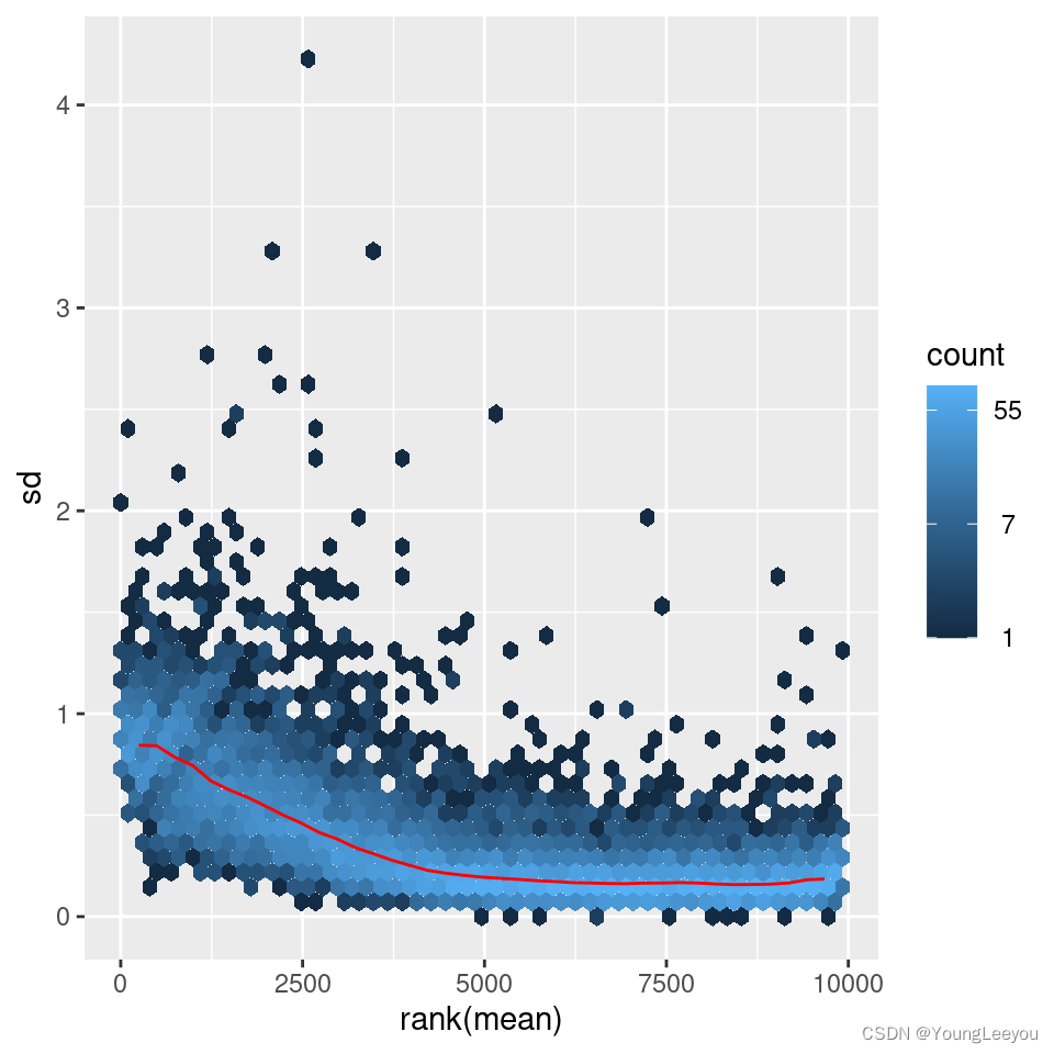
meanSdPlot(assay(vsd))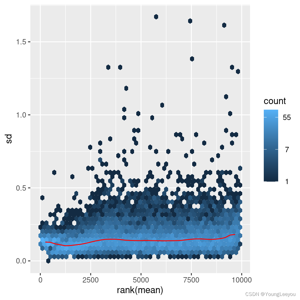
meanSdPlot(assay(rld))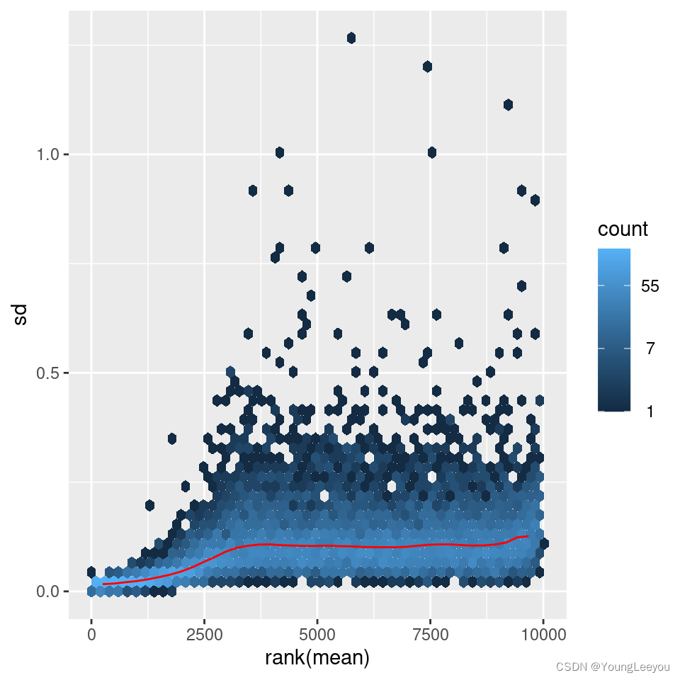
Data quality assessment by sample clustering and visualization
Data quality assessment and quality control (i.e. the removal of insufficiently good data) are essential steps of any data analysis. These steps should typically be performed very early in the analysis of a new data set, preceding or in parallel to the differential expression testing.
We define the term quality as fitness for purpose. Our purpose is the detection of differentially expressed genes, and we are looking in particular for samples whose experimental treatment suffered from an anormality that renders the data points obtained from these particular samples detrimental to our purpose.
Heatmap of the count matrix
To explore a count matrix, it is often instructive to look at it as a heatmap. Below we show how to produce such a heatmap for various transformations of the data.
library("pheatmap")
select <- order(rowMeans(counts(dds,normalized=TRUE)),
                decreasing=TRUE)[1:20]
df <- as.data.frame(colData(dds)[,c("condition","type")])
pheatmap(assay(ntd)[select,], cluster_rows=FALSE, show_rownames=FALSE,
         cluster_cols=FALSE, annotation_col=df)
pheatmap(assay(vsd)[select,], cluster_rows=FALSE, show_rownames=FALSE,
         cluster_cols=FALSE, annotation_col=df)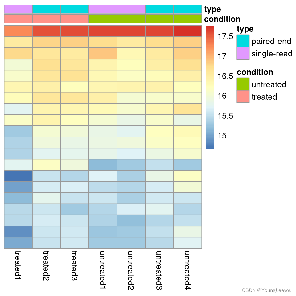
pheatmap(assay(rld)[select,], cluster_rows=FALSE, show_rownames=FALSE,
         cluster_cols=FALSE, annotation_col=df)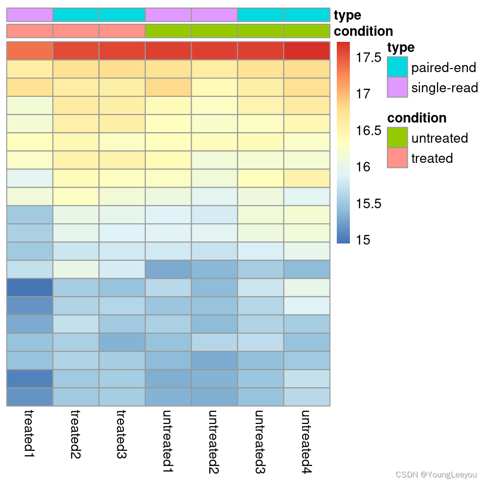
Heatmap of the sample-to-sample distances
Another use of the transformed data is sample clustering. Here, we apply the dist function to the transpose of the transformed count matrix to get sample-to-sample distances.
sampleDists <- dist(t(assay(vsd)))A heatmap of this distance matrix gives us an overview over similarities and dissimilarities between samples. We have to provide a hierarchical clustering hc to the heatmap function based on the sample distances, or else the heatmap function would calculate a clustering based on the distances between the rows/columns of the distance matrix.
library("RColorBrewer")
sampleDistMatrix <- as.matrix(sampleDists)
rownames(sampleDistMatrix) <- paste(vsd$condition, vsd$type, sep="-")
colnames(sampleDistMatrix) <- NULL
colors <- colorRampPalette( rev(brewer.pal(9, "Blues")) )(255)
pheatmap(sampleDistMatrix,
         clustering_distance_rows=sampleDists,
         clustering_distance_cols=sampleDists,
         col=colors)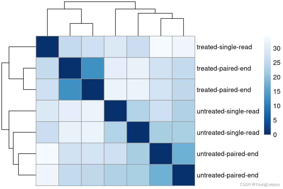
Principal component plot of the samples
Related to the distance matrix is the PCA plot, which shows the samples in the 2D plane spanned by their first two principal components. This type of plot is useful for visualizing the overall effect of experimental covariates and batch effects.
plotPCA(vsd, intgroup=c("condition", "type"))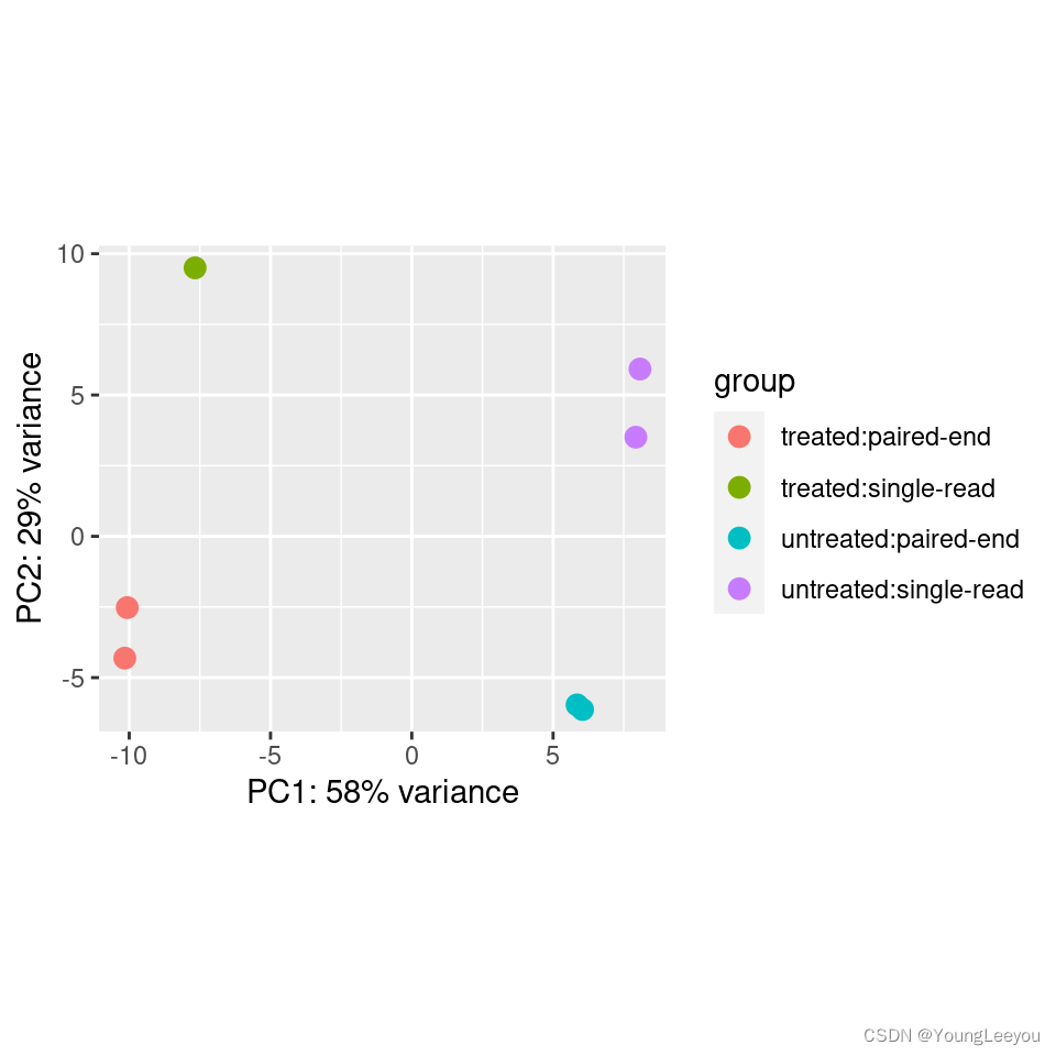
It is also possible to customize the PCA plot using the ggplot function.
pcaData <- plotPCA(vsd, intgroup=c("condition", "type"), returnData=TRUE)
percentVar <- round(100 * attr(pcaData, "percentVar"))
ggplot(pcaData, aes(PC1, PC2, color=condition, shape=type)) +
  geom_point(size=3) +
  xlab(paste0("PC1: ",percentVar[1],"% variance")) +
  ylab(paste0("PC2: ",percentVar[2],"% variance")) +
  coord_fixed()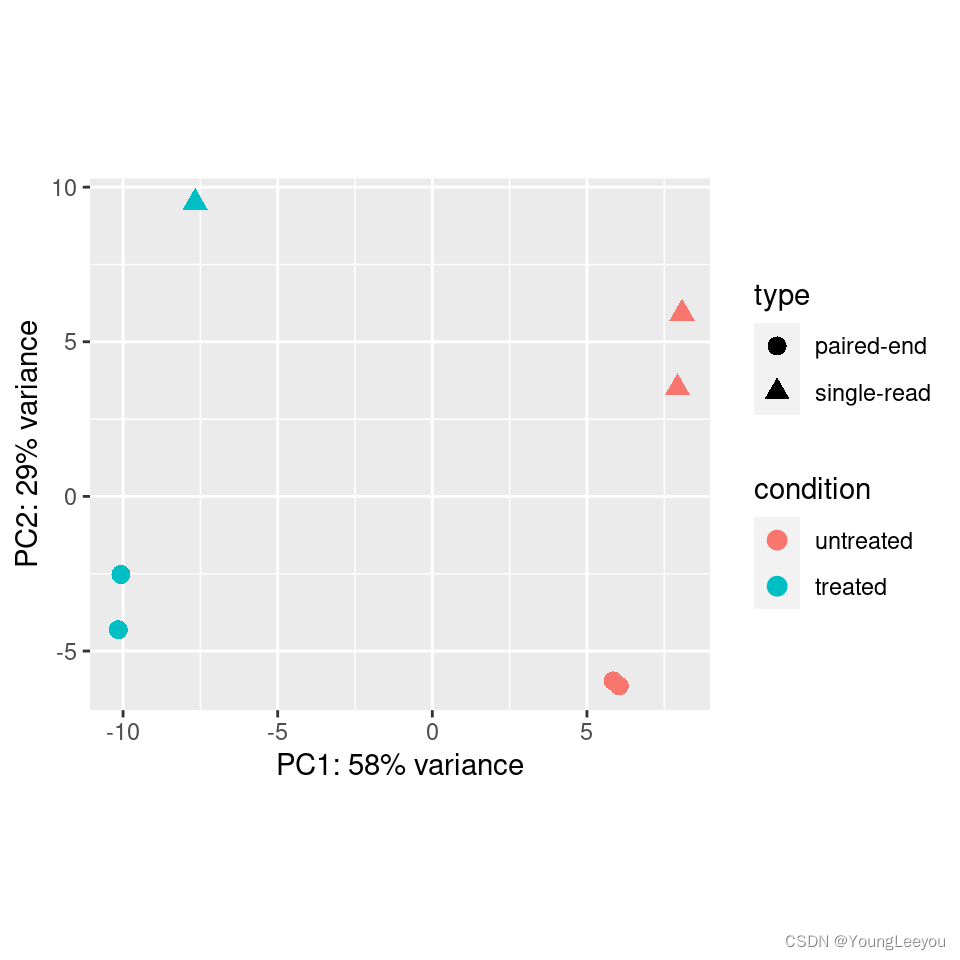
Variations to the standard workflow
Wald test individual steps
The function DESeq runs the following functions in order:
dds <- estimateSizeFactors(dds)
dds <- estimateDispersions(dds)
dds <- nbinomWaldTest(dds)
Contrasts
A contrast is a linear combination of estimated log2 fold changes, which can be used to test if differences between groups are equal to zero. The simplest use case for contrasts is an experimental design containing a factor with three levels, say A, B and C. Contrasts enable the user to generate results for all 3 possible differences: log2 fold change of B vs A, of C vs A, and of C vs B. The contrast argument of results function is used to extract test results of log2 fold changes of interest, for example:
results(dds, contrast=c("condition","C","B"))Log2 fold changes can also be added and subtracted by providing a list to the contrast argument which has two elements: the names of the log2 fold changes to add, and the names of the log2 fold changes to subtract. The names used in the list should come from resultsNames(dds). Alternatively, a numeric vector of the length of resultsNames(dds) can be provided, for manually specifying the linear combination of terms. A tutorial describing the use of numeric contrasts for DESeq2 explains a general approach to comparing across groups of samples. Demonstrations of the use of contrasts for various designs can be found in the examples section of the help page ?results. The mathematical formula that is used to generate the contrasts can be found below.
Interactions
Interaction terms can be added to the design formula, in order to test, for example, if the log2 fold change attributable to a given condition is different based on another factor, for example if the condition effect differs across genotype.
Initial note: Many users begin to add interaction terms to the design formula, when in fact a much simpler approach would give all the results tables that are desired. We will explain this approach first, because it is much simpler to perform. If the comparisons of interest are, for example, the effect of a condition for different sets of samples, a simpler approach than adding interaction terms explicitly to the design formula is to perform the following steps:
- combine the factors of interest into a single factor with all combinations of the original factors
- change the design to include just this factor, e.g. ~ group
Using this design is similar to adding an interaction term, in that it models multiple condition effects which can be easily extracted with results. Suppose we have two factors genotype (with values I, II, and III) and condition (with values A and B), and we want to extract the condition effect specifically for each genotype. We could use the following approach to obtain, e.g. the condition effect for genotype I:
dds$group <- factor(paste0(dds$genotype, dds$condition))
design(dds) <- ~ group
dds <- DESeq(dds)
resultsNames(dds)
results(dds, contrast=c("group", "IB", "IA"))
Adding interactions to the design: The following two plots diagram genotype-specific condition effects, which could be modeled with interaction terms by using a design of ~genotype + condition + genotype:condition.
In the first plot (Gene 1), note that the condition effect is consistent across genotypes. Although condition A has a different baseline for I,II, and III, the condition effect is a log2 fold change of about 2 for each genotype. Using a model with an interaction term genotype:condition, the interaction terms for genotype II and genotype III will be nearly 0.
Here, the y-axis represents log2(n+1), and each group has 20 samples (black dots). A red line connects the mean of the groups within each genotype.
## Warning: `fun.y` is deprecated. Use `fun` instead.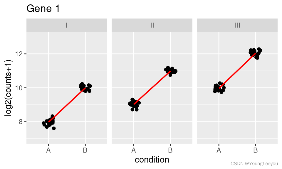
In the second plot (Gene 2), we can see that the condition effect is not consistent across genotype. Here the main condition effect (the effect for the reference genotype I) is again 2. However, this time the interaction terms will be around 1 for genotype II and -4 for genotype III. This is because the condition effect is higher by 1 for genotype II compared to genotype I, and lower by 4 for genotype III compared to genotype I. The condition effect for genotype II (or III) is obtained by adding the main condition effect and the interaction term for that genotype. Such a plot can be made using the plotCounts function as shown above.
## Warning: `fun.y` is deprecated. Use `fun` instead.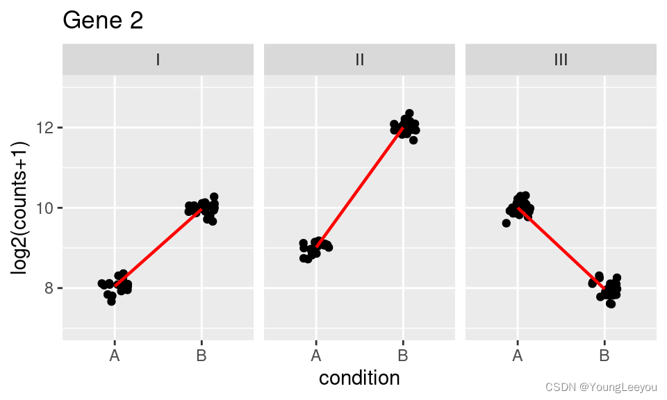
Now we will continue to explain the use of interactions in order to test for differences in condition effects. We continue with the example of condition effects across three genotypes (I, II, and III).
The key point to remember about designs with interaction terms is that, unlike for a design ~genotype + condition, where the condition effect represents the overall effect controlling for differences due to genotype, by adding genotype:condition, the main condition effect only represents the effect of condition for the reference level of genotype (I, or whichever level was defined by the user as the reference level). The interaction terms genotypeII.conditionB and genotypeIII.conditionB give the difference between the condition effect for a given genotype and the condition effect for the reference genotype.
This genotype-condition interaction example is examined in further detail in Example 3 in the help page for results, which can be found by typing ?results. In particular, we show how to test for differences in the condition effect across genotype, and we show how to obtain the condition effect for non-reference genotypes.
Time-series experiments
There are a number of ways to analyze time-series experiments, depending on the biological question of interest. In order to test for any differences over multiple time points, once can use a design including the time factor, and then test using the likelihood ratio test as described in the following section, where the time factor is removed in the reduced formula. For a control and treatment time series, one can use a design formula containing the condition factor, the time factor, and the interaction of the two. In this case, using the likelihood ratio test with a reduced model which does not contain the interaction terms will test whether the condition induces a change in gene expression at any time point after the reference level time point (time 0). An example of the later analysis is provided in our RNA-seq workflow.
Likelihood ratio test
DESeq2 offers two kinds of hypothesis tests: the Wald test, where we use the estimated standard error of a log2 fold change to test if it is equal to zero, and the likelihood ratio test (LRT). The LRT examines two models for the counts, a full model with a certain number of terms and a reduced model, in which some of the terms of the full model are removed. The test determines if the increased likelihood of the data using the extra terms in the full model is more than expected if those extra terms are truly zero.
The LRT is therefore useful for testing multiple terms at once, for example testing 3 or more levels of a factor at once, or all interactions between two variables. The LRT for count data is conceptually similar to an analysis of variance (ANOVA) calculation in linear regression, except that in the case of the Negative Binomial GLM, we use an analysis of deviance (ANODEV), where the deviance captures the difference in likelihood between a full and a reduced model.
The likelihood ratio test can be performed by specifying test="LRT" when using the DESeq function, and providing a reduced design formula, e.g. one in which a number of terms from design(dds) are removed. The degrees of freedom for the test is obtained from the difference between the number of parameters in the two models. A simple likelihood ratio test, if the full design was ~condition would look like:
dds <- DESeq(dds, test="LRT", reduced=~1)
res <- results(dds)
If the full design contained other variables, such as a batch variable, e.g. ~batch + condition then the likelihood ratio test would look like:
dds <- DESeq(dds, test="LRT", reduced=~batch)
res <- results(dds)
Extended section on shrinkage estimators
Here we extend the discussion of shrinkage estimators. Below is a summary table of differences between methods available in lfcShrink via the type argument (and for further technical reference on use of arguments please see ?lfcShrink):
| method: | apeglm1 | ashr2 | normal3 |
|---|---|---|---|
| Good for ranking by LFC | ✓ | ✓ | ✓ |
| Preserves size of large LFC | ✓ | ✓ | |
| Can compute s-values (Stephens 2016) | ✓ | ✓ | |
Allows use of coef | ✓ | ✓ | ✓ |
Allows use of lfcThreshold | ✓ | ✓ | |
Allows use of contrast | ✓ | ✓ | |
| Can shrink interaction terms | ✓ | ✓ |
References: 1. Zhu, Ibrahim, and Love (2018); 2. Stephens (2016); 3. Love, Huber, and Anders (2014)
Beginning with the first row, all shrinkage methods provided by DESeq2 are good for ranking genes by “effect size”, that is the log2 fold change (LFC) across groups, or associated with an interaction term. It is useful to contrast ranking by effect size with ranking by a p-value or adjusted p-value associated with a null hypothesis: while increasing the number of samples will tend to decrease the associated p-value for a gene that is differentially expressed, the estimated effect size or LFC becomes more precise. Also, a gene can have a small p-value although the change in expression is not great, as long as the standard error associated with the estimated LFC is small.
The next two rows point out that apeglm and ashr shrinkage methods help to preserve the size of large LFC, and can be used to compute s-values. These properties are related. As noted in the previous section, the original DESeq2 shrinkage estimator used a Normal distribution, with a scale that adapts to the spread of the observed LFCs. Because the tails of the Normal distribution become thin relatively quickly, it was important when we designed the method that the prior scaling is sensitive to the very largest observed LFCs. As you can read in the DESeq2 paper, under the section, “Empirical prior estimate”, we used the top 5% of the LFCs by absolute value to set the scale of the Normal prior (we later added weighting the quantile by precision). ashr, published in 2016, and apeglm use wide-tailed priors to avoid shrinking large LFCs. While a typical RNA-seq experiment may have many LFCs between -1 and 1, we might consider a LFC of >4 to be very large, as they represent 16-fold increases or decreases in expression. ashr and apeglm can adapt to the scale of the entirety of LFCs, while not over-shrinking the few largest LFCs. The potential for over-shrinking LFC is also why DESeq2’s shrinkage estimator is not recommended for designs with interaction terms.
What are s-values? This quantity proposed by Stephens (2016) gives the estimated rate of false sign among genes with equal or smaller s-value. Stephens (2016) points out they are analogous to the q-value of Storey (2003). The s-value has a desirable property relative to the adjusted p-value or q-value, in that it does not require supposing there to be a set of null genes with LFC = 0 (the most commonly used null hypothesis). Therefore, it can be benchmarked by comparing estimated LFC and s-value to the “true LFC” in a setting where this can be reasonably defined. For these estimated probabilities to be accurate, the scale of the prior needs to match the scale of the distribution of effect sizes, and so the original DESeq2 shrinkage method is not really compatible with computing s-values.
The last four rows explain differences in whether coefficients or contrasts can have shrinkage applied by the various methods. All three methods can use coef with either the name or numeric index from resultsNames(dds) to specify which coefficient to shrink. normal and apeglm also allow for a positive lfcThreshold to be specified, in which case, they will return p-values and adjusted p-values or s-values for the LFC being greater in absolute value than the threshold (see this section for normal). For apeglm, setting a threshold means that the s-values will give the “false sign or small” rate (FSOS) among genes with equal or small s-value. We found FSOS to be a useful description for when the LFC is either the wrong sign or less than the threshold distance from 0.
resApeT <- lfcShrink(dds, coef=2, type="apeglm", lfcThreshold=1)
plotMA(resApeT, ylim=c(-3,3), cex=.8)
abline(h=c(-1,1), col="dodgerblue", lwd=2)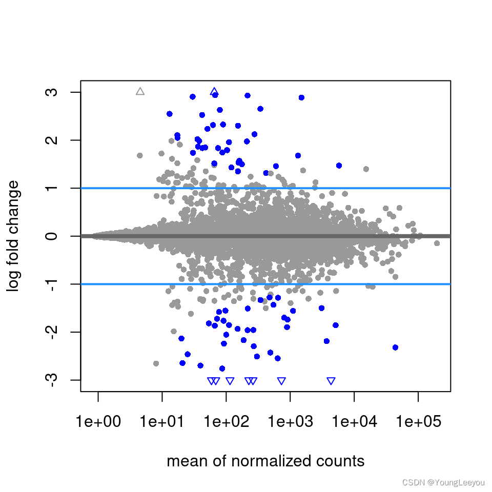
Finally, normal and ashr can be used with arbitrary specified contrast because normal shrinks multiple coefficients simultaneously (apeglm does not), and because ashr does not estimate a vector of coefficients but models estimated coefficients and their standard errors from upstream methods (here, DESeq2’s MLE). Although apeglm cannot be used with contrast, we note that many designs can be easily rearranged such that what was a contrast becomes its own coefficient. In this case, the dispersion does not have to be estimated again, as the designs are equivalent, up to the meaning of the coefficients. Instead, one need only run nbinomWaldTest to re-estimate MLE coefficients – these are necessary for apeglm – and then run lfcShrink specifying the coefficient of interest in resultsNames(dds).
We give some examples below of producing equivalent designs for use with coef. We show how the coefficients change with model.matrix, but the user would, for example, either change the levels of dds$condition or replace the design using design(dds)<-, then run nbinomWaldTest followed by lfcShrink.
Three groups:
condition <- factor(rep(c("A","B","C"),each=2))
model.matrix(~ condition)
## (Intercept) conditionB conditionC
## 1 1 0 0
## 2 1 0 0
## 3 1 1 0
## 4 1 1 0
## 5 1 0 1
## 6 1 0 1
## attr(,"assign")
## [1] 0 1 1
## attr(,"contrasts")
## attr(,"contrasts")$condition
## [1] "contr.treatment"# to compare C vs B, make B the reference level,
# and select the last coefficient
condition <- relevel(condition, "B")
model.matrix(~ condition)## (Intercept) conditionA conditionC
## 1 1 1 0
## 2 1 1 0
## 3 1 0 0
## 4 1 0 0
## 5 1 0 1
## 6 1 0 1
## attr(,"assign")
## [1] 0 1 1
## attr(,"contrasts")
## attr(,"contrasts")$condition
## [1] "contr.treatment"Three groups, compare condition effects:
grp <- factor(rep(1:3,each=4))
cnd <- factor(rep(rep(c("A","B"),each=2),3))
model.matrix(~ grp + cnd + grp:cnd)
## (Intercept) grp2 grp3 cndB grp2:cndB grp3:cndB
## 1 1 0 0 0 0 0
## 2 1 0 0 0 0 0
## 3 1 0 0 1 0 0
## 4 1 0 0 1 0 0
## 5 1 1 0 0 0 0
## 6 1 1 0 0 0 0
## 7 1 1 0 1 1 0
## 8 1 1 0 1 1 0
## 9 1 0 1 0 0 0
## 10 1 0 1 0 0 0
## 11 1 0 1 1 0 1
## 12 1 0 1 1 0 1
## attr(,"assign")
## [1] 0 1 1 2 3 3
## attr(,"contrasts")
## attr(,"contrasts")$grp
## [1] "contr.treatment"
##
## attr(,"contrasts")$cnd
## [1] "contr.treatment"# to compare condition effect in group 3 vs 2,
# make group 2 the reference level,
# and select the last coefficient
grp <- relevel(grp, "2")
model.matrix(~ grp + cnd + grp:cnd)## (Intercept) grp1 grp3 cndB grp1:cndB grp3:cndB
## 1 1 1 0 0 0 0
## 2 1 1 0 0 0 0
## 3 1 1 0 1 1 0
## 4 1 1 0 1 1 0
## 5 1 0 0 0 0 0
## 6 1 0 0 0 0 0
## 7 1 0 0 1 0 0
## 8 1 0 0 1 0 0
## 9 1 0 1 0 0 0
## 10 1 0 1 0 0 0
## 11 1 0 1 1 0 1
## 12 1 0 1 1 0 1
## attr(,"assign")
## [1] 0 1 1 2 3 3
## attr(,"contrasts")
## attr(,"contrasts")$grp
## [1] "contr.treatment"
##
## attr(,"contrasts")$cnd
## [1] "contr.treatment"Two groups, two individuals per group, compare within-individual condition effects:
grp <- factor(rep(1:2,each=4))
ind <- factor(rep(rep(1:2,each=2),2))
cnd <- factor(rep(c("A","B"),4))
model.matrix(~grp + grp:ind + grp:cnd)
## (Intercept) grp2 grp1:ind2 grp2:ind2 grp1:cndB grp2:cndB
## 1 1 0 0 0 0 0
## 2 1 0 0 0 1 0
## 3 1 0 1 0 0 0
## 4 1 0 1 0 1 0
## 5 1 1 0 0 0 0
## 6 1 1 0 0 0 1
## 7 1 1 0 1 0 0
## 8 1 1 0 1 0 1
## attr(,"assign")
## [1] 0 1 2 2 3 3
## attr(,"contrasts")
## attr(,"contrasts")$grp
## [1] "contr.treatment"
##
## attr(,"contrasts")$ind
## [1] "contr.treatment"
##
## attr(,"contrasts")$cnd
## [1] "contr.treatment"# to compare condition effect across group,
# add a main effect for 'cnd',
# and select the last coefficient
model.matrix(~grp + cnd + grp:ind + grp:cnd)## (Intercept) grp2 cndB grp1:ind2 grp2:ind2 grp2:cndB
## 1 1 0 0 0 0 0
## 2 1 0 1 0 0 0
## 3 1 0 0 1 0 0
## 4 1 0 1 1 0 0
## 5 1 1 0 0 0 0
## 6 1 1 1 0 0 1
## 7 1 1 0 0 1 0
## 8 1 1 1 0 1 1
## attr(,"assign")
## [1] 0 1 2 3 3 4
## attr(,"contrasts")
## attr(,"contrasts")$grp
## [1] "contr.treatment"
##
## attr(,"contrasts")$cnd
## [1] "contr.treatment"
##
## attr(,"contrasts")$ind
## [1] "contr.treatment"par(mar=c(8,5,2,2))
boxplot(log10(assays(dds)[["cooks"]]), range=0, las=2)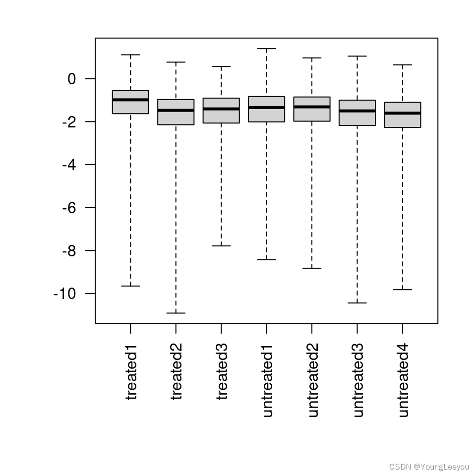


 被折叠的 条评论
为什么被折叠?
被折叠的 条评论
为什么被折叠?
 到【灌水乐园】发言


