scwgcna官网教程中英文实战高维wgcna分析单细胞wgcna分析-CSDN博客

本文链接：https://blog.csdn.net/qq_52813185/article/details/127780399

https://smorabit.github.io/hdWGCNA/index.html

https://mp.weixin.qq.com/s/OBvS0I7IUuwcChGoaJVgtQ

https://smorabit.github.io/hdWGCNA/articles/basic_tutorial.html#co-expression-network-analysis

load("D:/ARDS_scripts_1012/ARDS/Step2_harmony_f200_R3/0805/cluster_merge/sepsis_cluster_merge.rds")##	改路径
table(All.merge$stim)
table(Idents(All.merge),All.merge$stim)

1创建对象，选择基因

length(VariableFeatures(All.merge))

seurat_obj <- SetupForWGCNA(
  All.merge,
  gene_select = "fraction", # the gene selection approach
  fraction = 0.05, #  use genes that are expressed in a certain fraction of cells for in the whole dataset or in each group of cells, specified by group.by fraction of cells that a gene needs to be expressed in order to be included
  #variable=
  wgcna_name = "tutorial" # the name of the hdWGCNA experiment
)

length(seurat_obj@misc $t u t or ia l$ wgcna_genes) #[1] 5735

table(seurat_obj$cell.type)

table(seurat_obj$stim)

seurat_obj$Sample=seurat_obj$stim
seurat_obj$cell_type=seurat_obj$cell.type

在这里插入图片描述

2# construct metacells in each group

seurat_obj <- MetacellsByGroups(
  seurat_obj = seurat_obj,
  group.by = c("cell_type", "Sample"), # specify the columns in seurat_obj@meta.data to group by
  k = 20, # nearest-neighbors parameter
  reduction = "harmony", # 降维方法
  slot='counts',
  max_shared = 10, # maximum number of shared cells between two metacells
  ident.group = 'cell_type' # set the Idents of the metacell seurat object
)

3#标准化：NormalizeMetacells
#提取metacell：GetMetacellObject

# normalize metacell expression matrix:
seurat_obj <- NormalizeMetacells(seurat_obj)
#  get the metacell object from the hdWGCNA experiment
metacell_obj <- GetMetacellObject(seurat_obj)
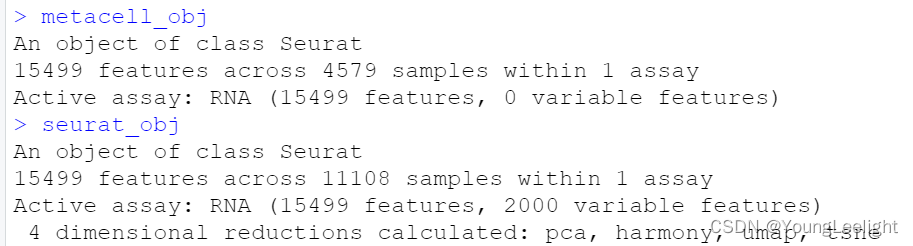
metacell_obj
seurat_obj
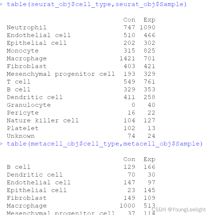
table(seurat_obj$cell_type,seurat_obj$Sample)
table(metacell_obj$cell_type,metacell_obj$Sample)

在这里插入图片描述

3.1#可选，是否处理metacell 进行可视化

if(F){
  seurat_obj <- NormalizeMetacells(seurat_obj)
  seurat_obj <- ScaleMetacells(seurat_obj, features=VariableFeatures(seurat_obj))
  seurat_obj <- RunPCAMetacells(seurat_obj, features=VariableFeatures(seurat_obj))
  seurat_obj <- RunHarmonyMetacells(seurat_obj, group.by.vars='Sample')
  seurat_obj <- RunUMAPMetacells(seurat_obj, reduction='harmony', dims=1:15)
  
  
  p1 <- DimPlotMetacells(seurat_obj, group.by='cell_type') + umap_theme() + ggtitle("Cell Type")
  p2 <- DimPlotMetacells(seurat_obj, group.by='Sample') + umap_theme() + ggtitle("Sample")
  
  p1 | p2
  
}

4#共表达网络分析

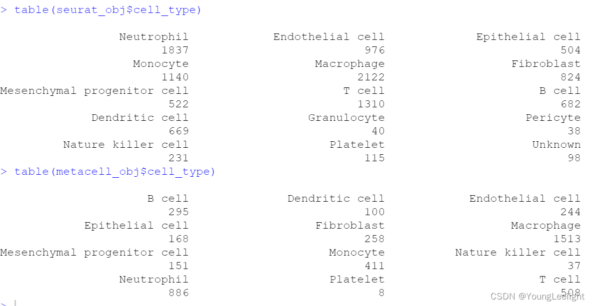
table(seurat_obj$cell_type)
table(metacell_obj$cell_type)

在这里插入图片描述

4.1#提取感兴趣的细胞亚群如果是多个亚群

group_name = c("INH", "EX")

seurat_obj <- SetDatExpr(
  seurat_obj,
  group_name = c("Monocyte","Macrophage","Dendritic cell","Neutrophil",
                 "T cell","Fibroblast","Endothelial cell",
                 "Epithelial cell","B cell",
                 "Mesenchymal progenitor cell"), # the name of the group of interest in the group.by column
  group.by='cell_type', # the metadata column containing the cell type info. This same column should have also been used in MetacellsByGroups
  assay = 'RNA', # using RNA assay
  use_metacells = TRUE, # use the metacells (TRUE) or the full expression matrix (FALSE)
  slot = 'data' # using normalized data
)

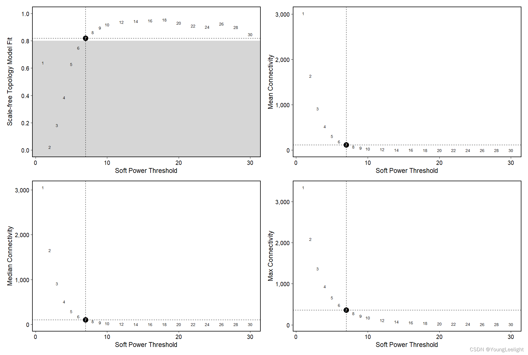
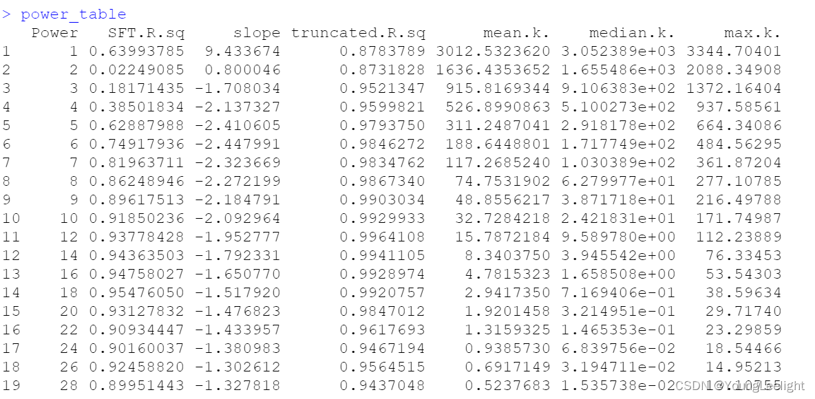
4.2#选取软阈值软阈值可以自动函数选择，也可以人工指定selected_power = NULL进行绘图

Test different soft powers:

seurat_obj <- TestSoftPowers(
  seurat_obj,
  setDatExpr=FALSE,
  powers = c(seq(1, 10, by = 1), seq(12, 30, by = 2))) # 选取soft powers(默认)
# networkType = 'signed' # 网络类型 "unsigned" or "signed hybrid"

# plot the results:
plot_list <- PlotSoftPowers(seurat_obj,
                            point_size = 5,
                            text_size = 3)
# assemble with patchwork
wrap_plots(plot_list, ncol=2) 
# plot the results:
plot_list <- PlotSoftPowers(seurat_obj)
# assemble with patchwork
wrap_plots(plot_list, ncol=2)

在这里插入图片描述

power_table <- GetPowerTable(seurat_obj)
head(power_table)

在这里插入图片描述

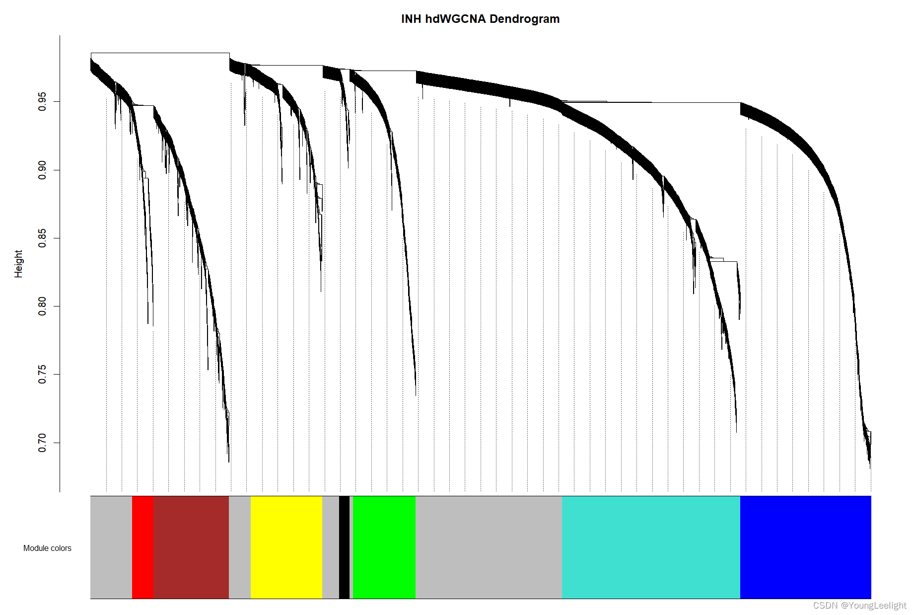
4.3#拓扑重叠矩阵（TOM） Construct co-expression network

seurat_obj <- ConstructNetwork(
  seurat_obj, 
  soft_power=7, # 因为上面一张图看上去7比较好
  setDatExpr=FALSE,
  corType = "pearson",
  networkType = "signed",
  TOMType = "signed",
  detectCutHeight = 0.995,
  minModuleSize = 50,
  mergeCutHeight = 0.2,
  tom_outdir = "TOM", # 输出文件夹
  tom_name = 'many_celltypes' # name of the topoligical overlap matrix written to disk
)
PlotDendrogram(seurat_obj, main='INH hdWGCNA Dendrogram')

在这里插入图片描述

4.3.1 可选
#TOM <- GetTOM(seurat_obj)

4.4#计算ME值

DefaultAssay(seurat_obj)
length(VariableFeatures(seurat_obj))

# need to run ScaleData first or else harmony throws an error:
seurat_obj <- ScaleData(seurat_obj, features=VariableFeatures(seurat_obj))

# compute all MEs in the full single-cell dataset
seurat_obj <- ModuleEigengenes(
  seurat_obj,
  scale.model.use = "linear", #  choices are "linear", "poisson", or "negbinom"
  assay = NULL, # 默认:DefaultAssay(seurat_obj)
  pc_dim = 1,
  group.by.vars="Sample" # 根据样本去批次化 harmonize
)

# harmonized module eigengenes:
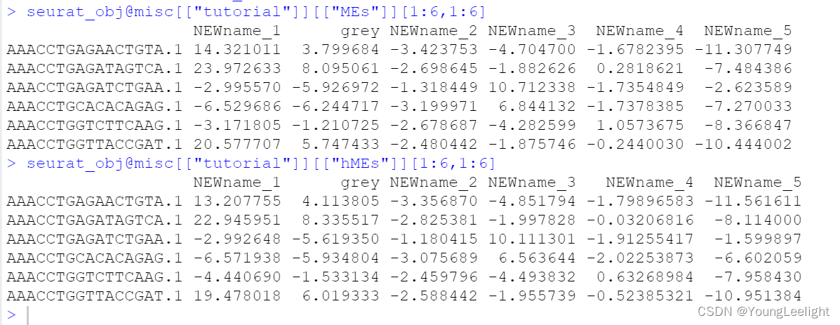
hMEs <- GetMEs(seurat_obj)

# module eigengenes:
MEs <- GetMEs(seurat_obj, harmonized=FALSE)

colnames(seurat_obj@misc[["tutorial"]][["hMEs"]])
seurat_obj@misc[["tutorial"]][["MEs"]][1:6,1:6]
seurat_obj@misc[["tutorial"]][["hMEs"]][1:6,1:6]

这里的列名是被后面重新命名的本来是颜色的标签
在这里插入图片描述

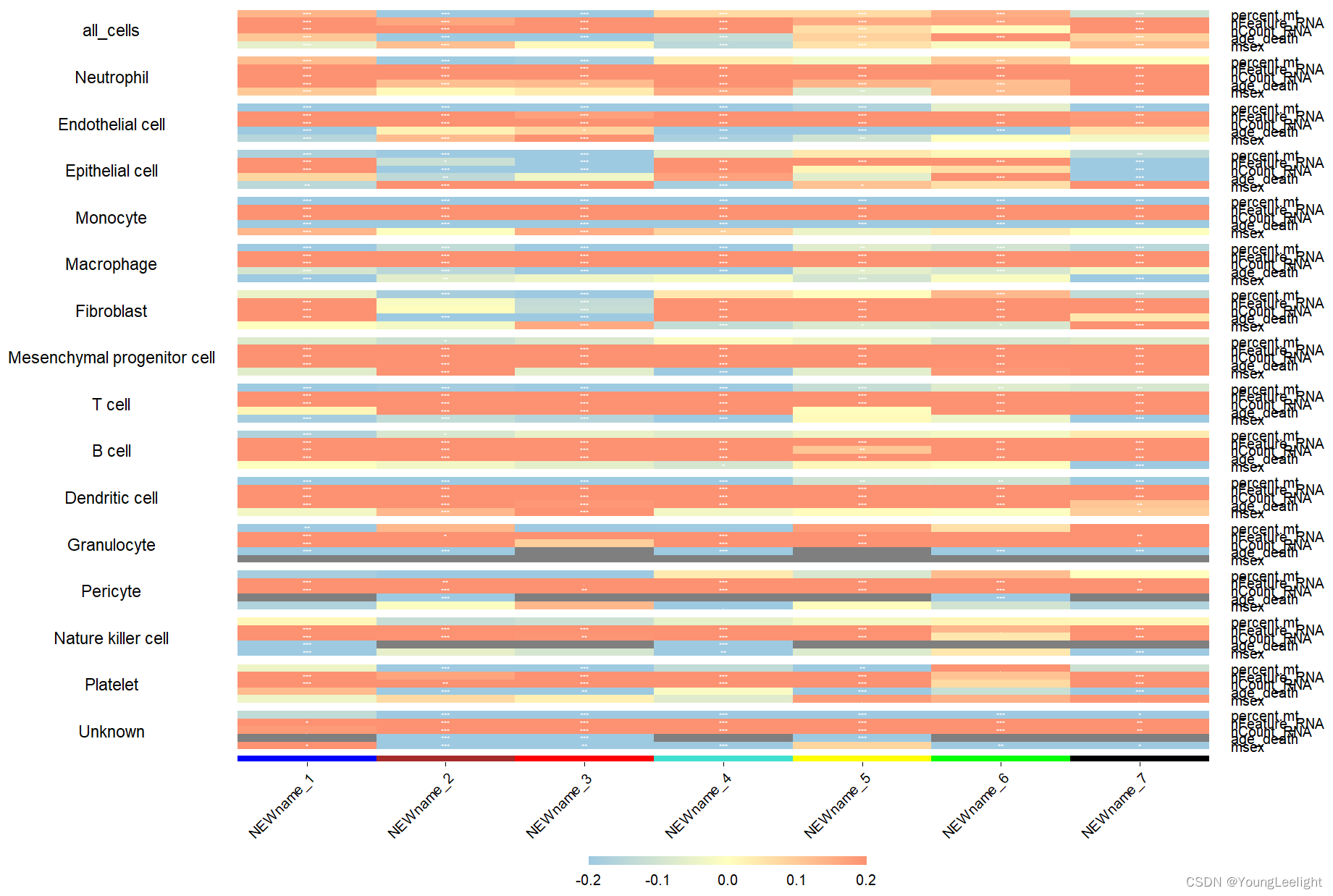
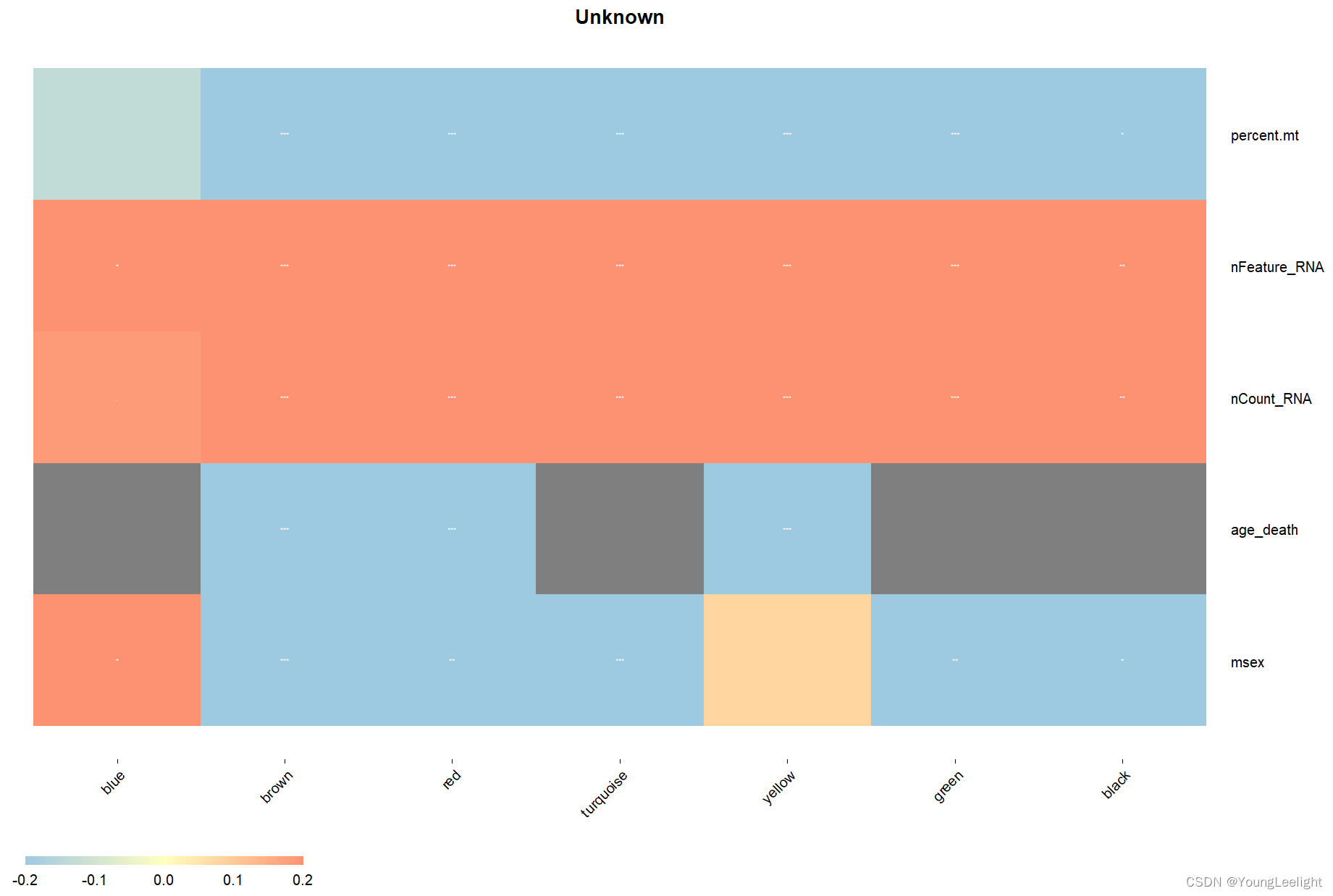
4.5#模块与性状间的相关性
#其实本质上还是设置成二分类变量或者数字，这样得到的结果就具有生物学意义

if(T){
  # convert sex to factor
  seurat_obj$msex <- as.factor(seurat_obj$stim)
  
  # convert age_death to numeric
  seurat_obj$age_death <- as.numeric(seurat_obj$seurat_clusters)
  # list of traits to correlate
  head(seurat_obj@meta.data)
  cur_traits <- c( 'msex', 'age_death',  
                   'nCount_RNA', 'nFeature_RNA', 'percent.mt')
  
  str(seurat_obj@meta.data[,cur_traits])
  # 使用去批次化后的hME
  seurat_obj <- ModuleTraitCorrelation(
    seurat_obj,
    traits = cur_traits,
    features = "hMEs", # Valid choices are hMEs, MEs, or scores
    cor_method = "pearson", # Valid choices are pearson, spearman, kendall.
    group.by='cell_type'
  )
  # get the mt-correlation results
  mt_cor <- GetModuleTraitCorrelation(seurat_obj)

names(mt_cor)

“cor” “pval” “fdr”

 PlotModuleTraitCorrelation(
    seurat_obj,
    label = 'fdr', # add p-val label in each cell of the heatmap
    label_symbol = 'stars', # labels as 'stars' or as 'numeric'
    text_size = 2,
    text_digits = 2,
    text_color = 'white',
    high_color = '#fc9272',
    mid_color = '#ffffbf',
    low_color = '#9ecae1',
    plot_max = 0.2,
    combine=T # 合并结果
  )
  PlotModuleTraitCorrelation(
    seurat_obj,
    label = 'fdr', # add p-val label in each cell of the heatmap
    label_symbol = 'stars', # labels as 'stars' or as 'numeric'
    text_size = 2,
    text_digits = 2,
    text_color = 'white',
    high_color = '#fc9272',
    mid_color = '#ffffbf',
    low_color = '#9ecae1',
    plot_max = 0.2,
    combine=F # 合并结果
  )

}
在这里插入图片描述

4.6 #hubgenes和功能评分 compute eigengene-based connectivity (kME):

# compute eigengene-based connectivity (kME):
seurat_obj <- ModuleConnectivity(
  seurat_obj,
  group.by = 'cell_type', 
  corFnc = "bicor", # to obtain Pearson correlation
  corOptions = "use='p'", # to obtain Pearson correlation
  harmonized = TRUE,
  assay = NULL,
  slot = "data", # default to normalized 'data' slot
  group_name = c("Monocyte","Macrophage","Dendritic cell","Neutrophil",
                 "T cell","Fibroblast","Endothelial cell",
                 "Epithelial cell","B cell",
                 "Mesenchymal progenitor cell") # 感兴趣的细胞群
)

rename the modules

# 改名后后模块赋予新的名称，以new_name为基础，后续附加个数字
seurat_obj <- ResetModuleNames( #https://smorabit.github.io/hdWGCNA/articles/customization.html
  seurat_obj,
  new_name = "NEWname_"  # the base name for the new modules
)

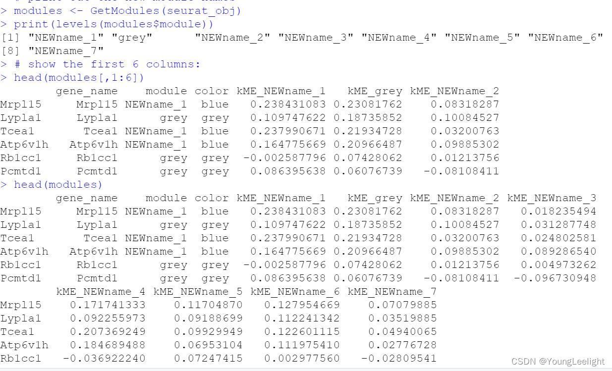
print out the new module names

modules <- GetModules(seurat_obj)

print(levels(modules$module))

# show the first 6 columns:
head(modules[,1:6])

在这里插入图片描述

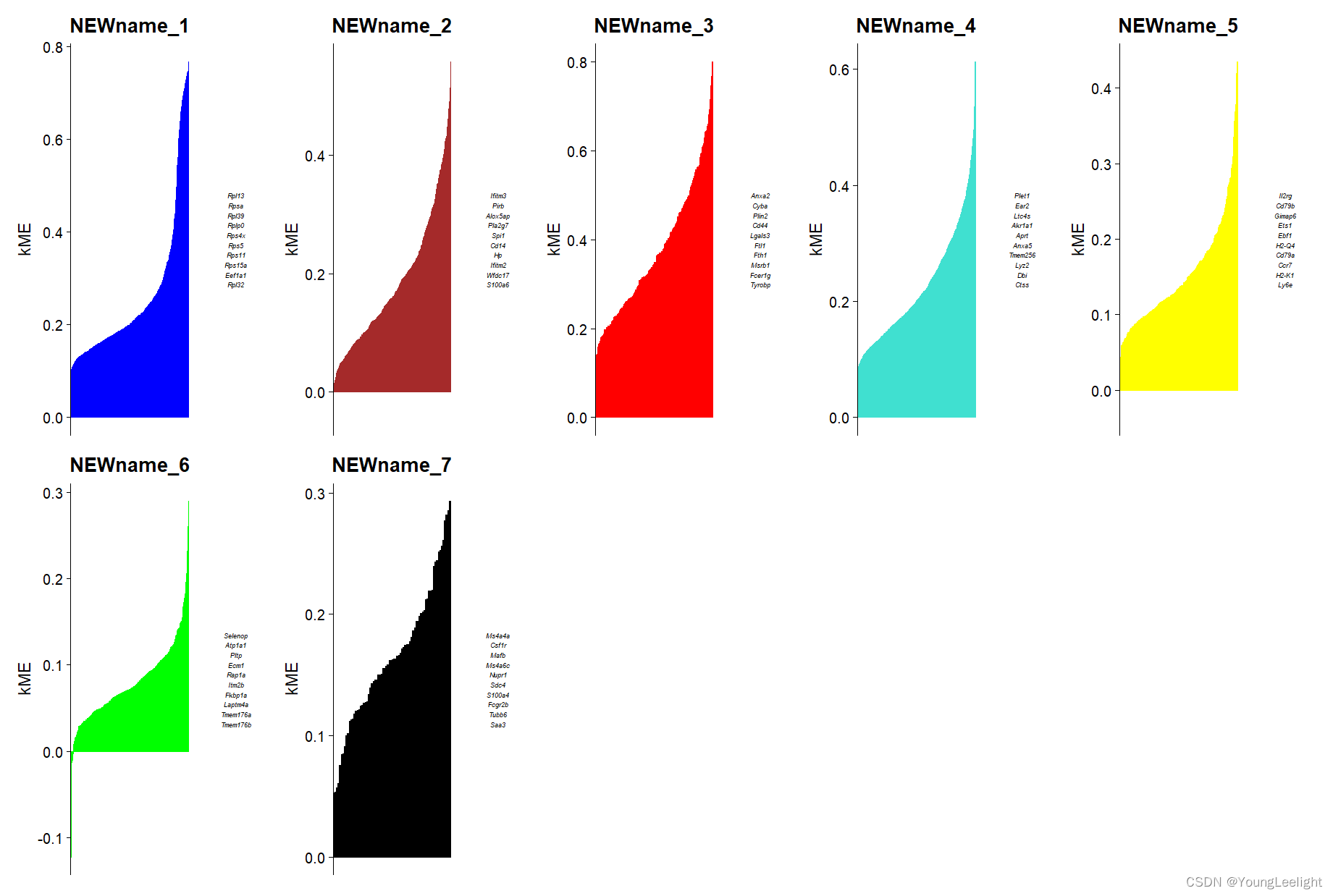
plot genes ranked by kME for each module

p <- PlotKMEs(seurat_obj, 
              ncol=5,
              n_hubs = 10, # number of hub genes to display
              text_size = 2,
              plot_widths = c(3, 2) # the relative width between the kME rank plot and the hub gene text
)
p

在这里插入图片描述

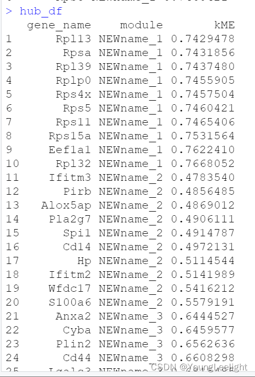
get hub genes

hub_df <- GetHubGenes(seurat_obj, n_hubs = 10)

head(hub_df)

在这里插入图片描述

dir.create(“./data”)

saveRDS(seurat_obj, file=‘data/hdWGCNA_object.rds’)

4.6.2 #基因功能评分

# compute gene scoring for the top 25 hub genes by kME for each module
# with Seurat method
seurat_obj <- ModuleExprScore(
  seurat_obj,
  n_genes = 25,
  method='Seurat'
)

compute gene scoring for the top 25 hub genes by kME for each module

with UCell method

library(UCell)
seurat_obj <- ModuleExprScore(
  seurat_obj,
  n_genes = 25,
  method='UCell'
)

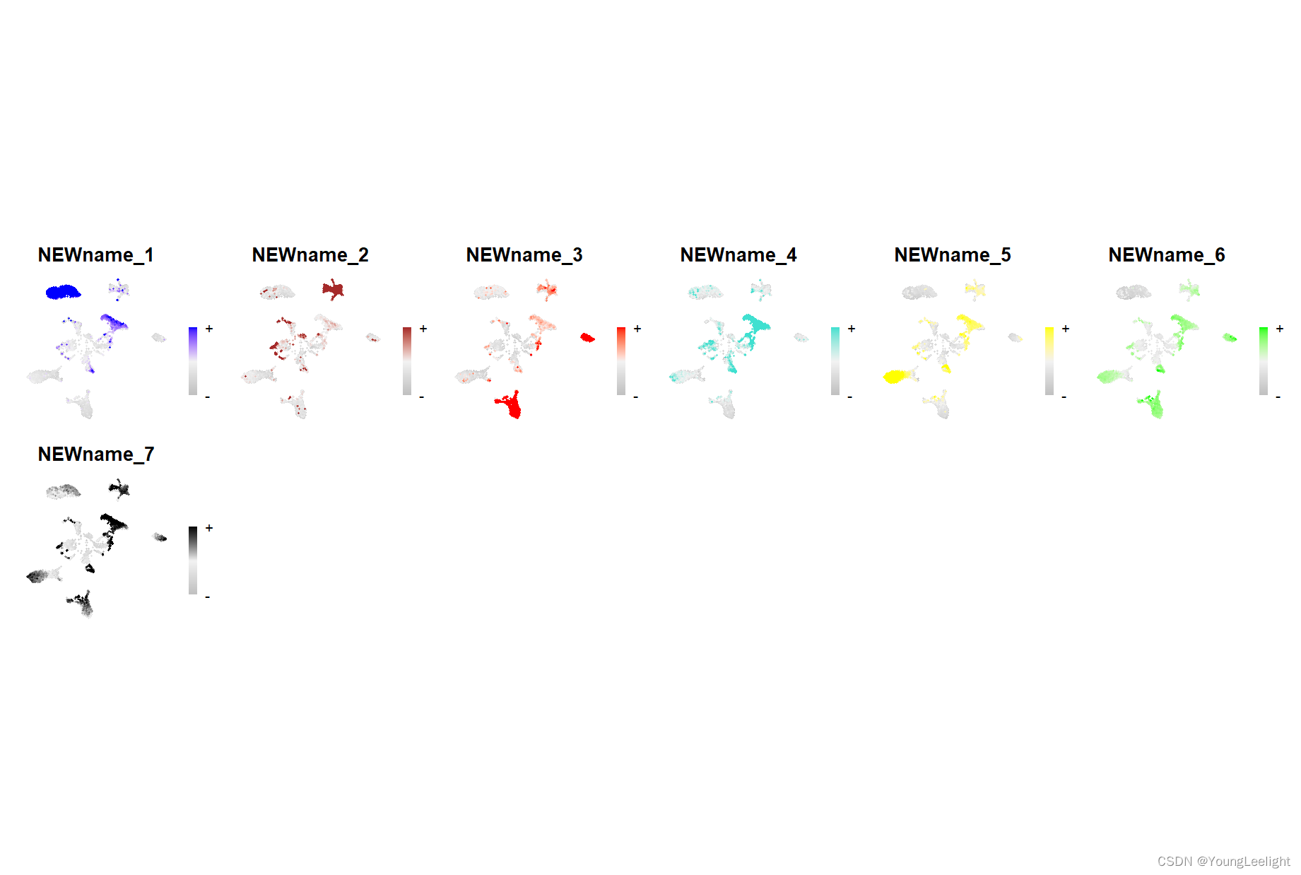
4.7#可视化

 make a featureplot of hMEs for each module
#其实features可以展示四种分数（hMEs, MEs, scores, or average）
plot_list <-ModuleFeaturePlot(
  seurat_obj,
  reduction = "umap",
  features = "hMEs",
  #features='scores', # plot the hub gene scores
  order_points = TRUE, # order so the points with highest hMEs are on top
  restrict_range = TRUE,
  point_size = 0.5,
  alpha = 1,
  label_legend = FALSE,
  raster_dpi = 500,
  raster_scale = 1,
  plot_ratio = 1,
  title = TRUE
)

stitch together with patchwork

wrap_plots(plot_list, ncol=6)

在这里插入图片描述

# make a featureplot of hub scores for each module
plot_list <- ModuleFeaturePlot(
  seurat_obj,
  features='scores', # plot the hub gene scores
  order='shuffle', # order so cells are shuffled
  ucell = TRUE # depending on Seurat vs UCell for gene scoring
)

在这里插入图片描述

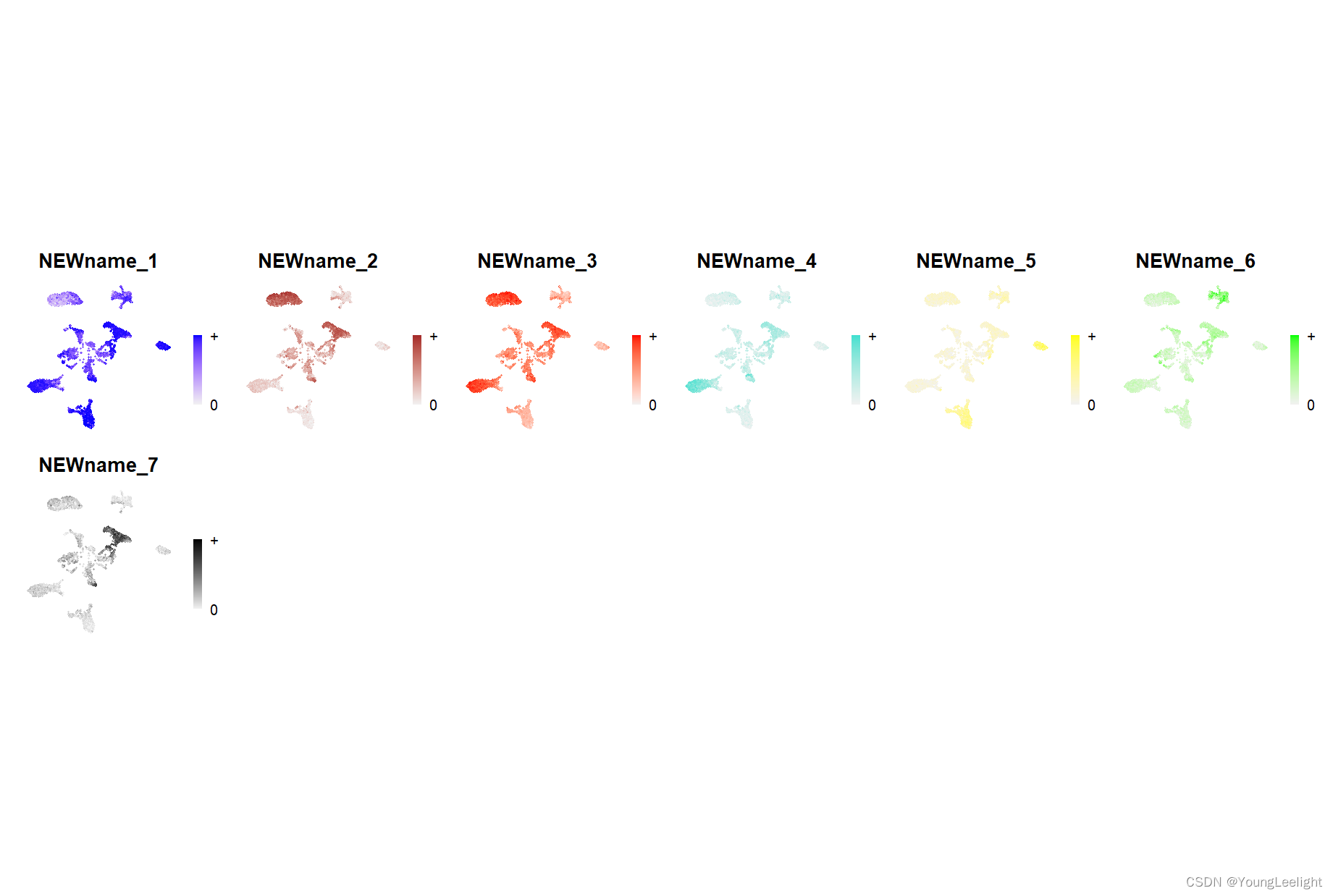
stitch together with patchwork

wrap_plots(plot_list, ncol=6)

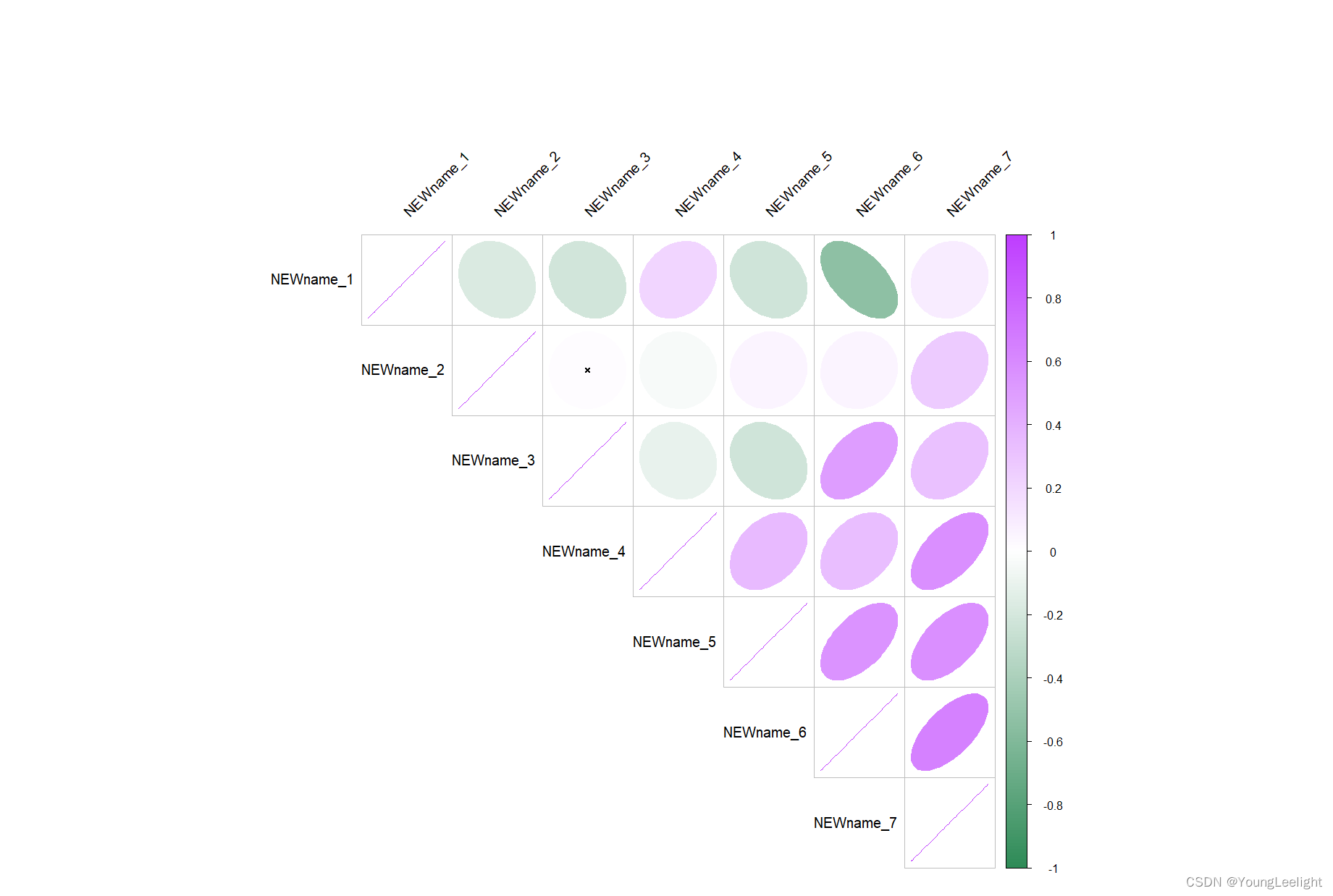
4.71 模块间相关性

# plot module correlagram
ModuleCorrelogram(seurat_obj,
                  exclude_grey = TRUE, # 默认删除灰色模块
                  features = "hMEs" # What to plot? Can select hMEs, MEs, scores, or average
)

在这里插入图片描述

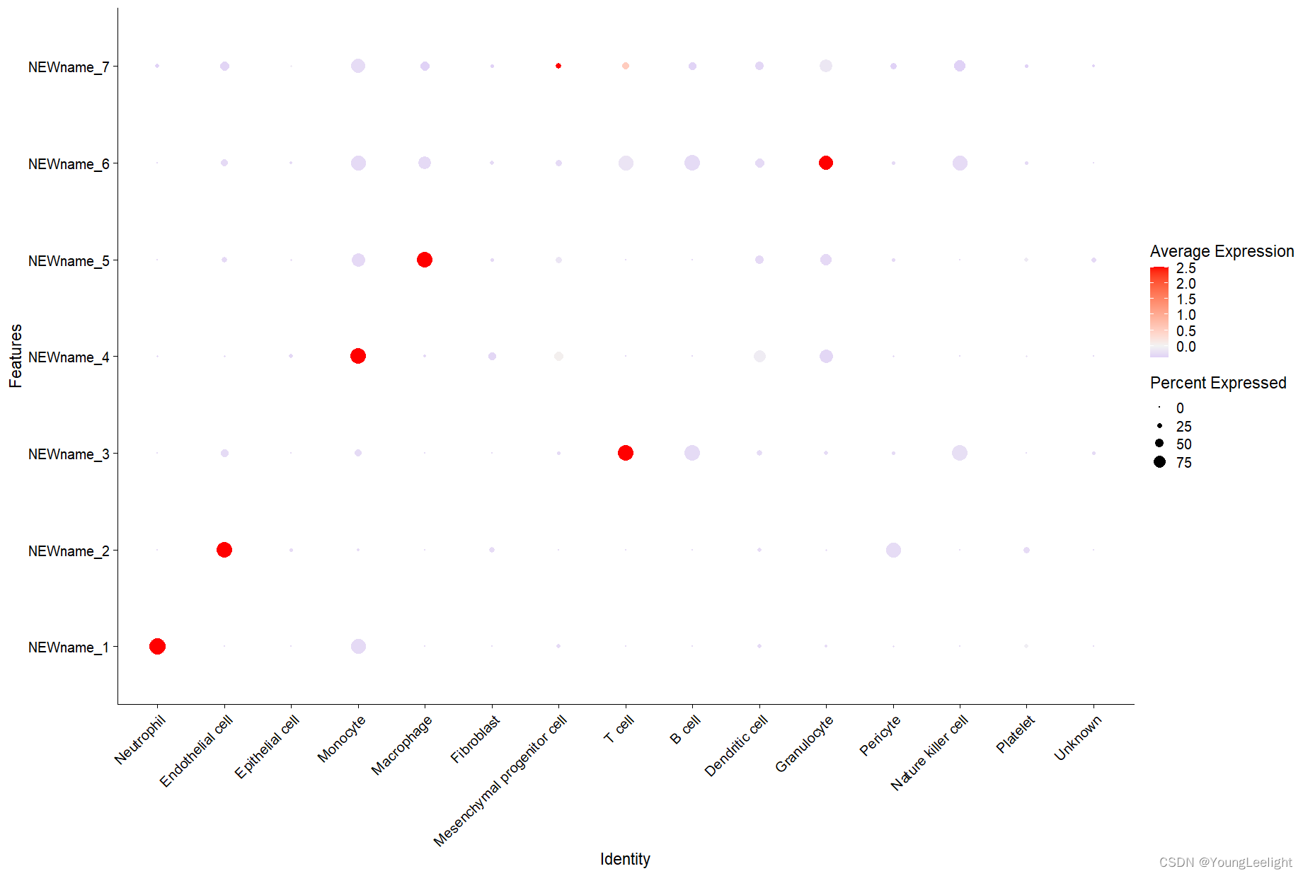
气泡图

# get hMEs from seurat object
MEs <- GetMEs(seurat_obj, harmonized=TRUE)
mods <- colnames(MEs); mods <- mods[mods != 'grey']

# add hMEs to Seurat meta-data:
seurat_obj@meta.data <- cbind(seurat_obj@meta.data, MEs)
# plot with Seurat's DotPlot function
p <- DotPlot(seurat_obj, features=mods, group.by = 'cell_type')

# flip the x/y axes, rotate the axis labels, and change color scheme:
p <- p +
  coord_flip() +
  RotatedAxis() +
  scale_color_gradient2(high='red', mid='grey95', low='blue')

# plot output
p

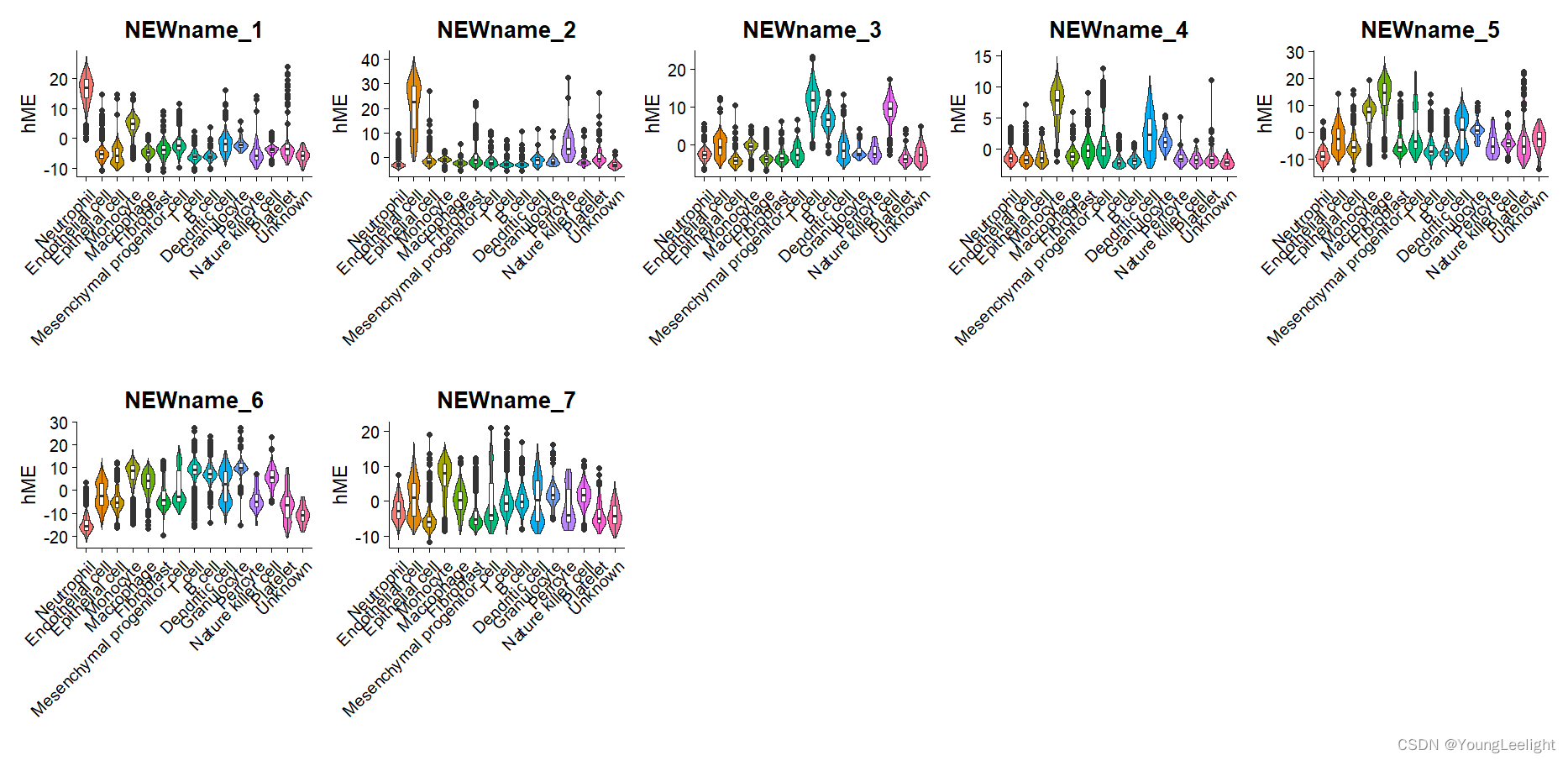
#气泡图

if(T){# Plot INH-M4 hME using Seurat VlnPlot function
  p <- VlnPlot(
    seurat_obj,
    features = 'NEWname_2',
    group.by = 'cell_type',
    pt.size = 0 # don't show actual data points
  )
  
  # add box-and-whisker plots on top:
  p <- p + geom_boxplot(width=.25, fill='white')
  
  # change axis labels and remove legend:
  p <- p + xlab('') + ylab('hME') + NoLegend()
  
  # plot output
  p
  }

在这里插入图片描述

#批量出图

plot_list <- lapply(mods, function(x) {
  print(x)
  p <- VlnPlot(
    seurat_obj,
    features = x,
    group.by = 'cell_type',
    pt.size = 0 # don't show actual data points
  )
  
  # add box-and-whisker plots on top:
  p <- p + geom_boxplot(width=.25, fill='white')
  
  # change axis labels and remove legend:
  p <- p + xlab('') + ylab('hME') + NoLegend()
  
  p
})
wrap_plots(plot_list, ncol = 5)

请添加图片描述

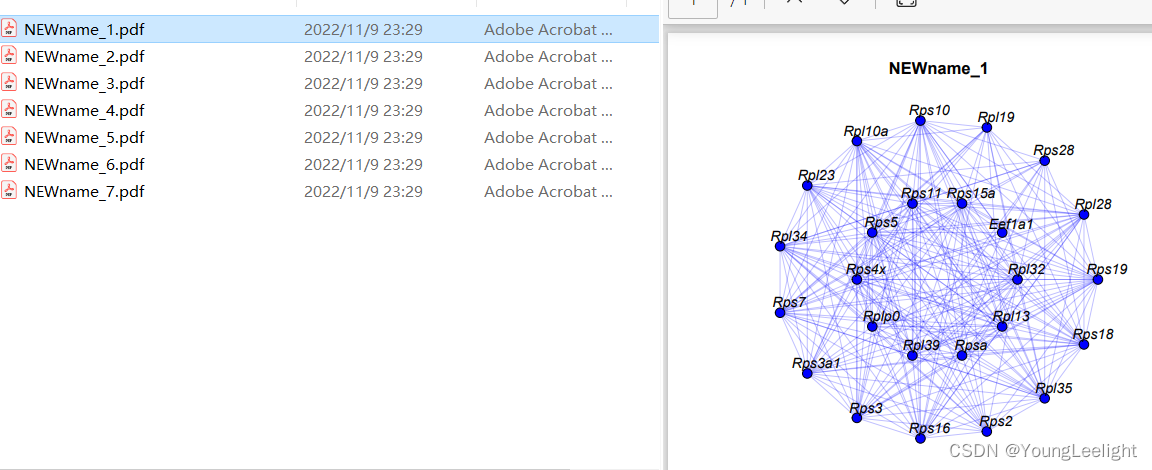
网络可视化
单个模块网络图

library(igraph)
# Visualizes the top hub genes for selected modules as a circular network plot
ModuleNetworkPlot(
  seurat_obj,
  mods = "all", # all modules are plotted.
  outdir = "ModuleNetworks", # The directory where the plots will be stored.
  plot_size = c(6, 6),
  label_center = FALSE,
  edge.alpha = 0.25,
  vertex.label.cex = 1, # 基因标签的字体大小
  vertex.size = 6 # 节点的大小
)

在这里插入图片描述

组合网络图

hubgene network

HubGeneNetworkPlot(
  seurat_obj,
  mods = "all", # all modules are plotted.
  n_hubs = 3, 
  n_other=6,
  edge_prop = 0.75,
)

g <- HubGeneNetworkPlot(seurat_obj,  return_graph=TRUE)


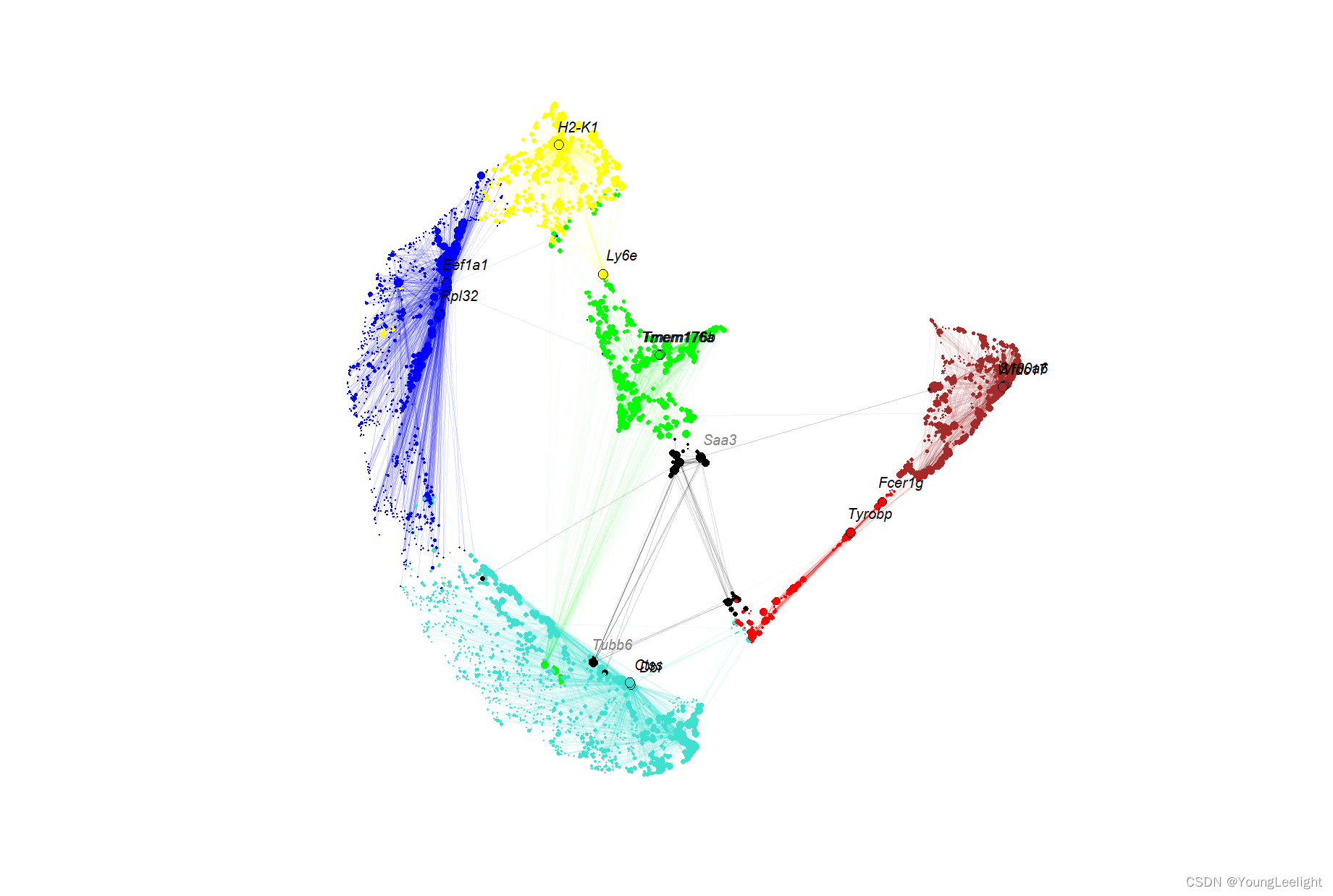
#umap网络图
这里使用另一种方法umap来可视化共表达网络中的所有基因，主要在topological overlap matrix (TOM)矩阵计算出umap坐标
seurat_obj <- RunModuleUMAP(
  seurat_obj,
  n_hubs = 10, # number of hub genes to include for the UMAP embedding
  n_neighbors=15, # neighbors parameter for UMAP
  min_dist=0.1 # min distance between points in UMAP space
)

# get the hub gene UMAP table from the seurat object
umap_df <- GetModuleUMAP(seurat_obj)

# plot with ggplot
ggplot(umap_df, aes(x=UMAP1, y=UMAP2)) +
  geom_point(
    color=umap_df$color, # color each point by WGCNA module
    size=umap_df$kME*2 # size of each point based on intramodular connectivity
  ) +
  umap_theme()

ModuleUMAPPlot(
  seurat_obj,
  edge.alpha=0.25,
  sample_edges=TRUE,
  edge_prop=0.1, # proportion of edges to sample (20% here)
  label_hubs=2 ,# how many hub genes to plot per module?
  keep_grey_edges=FALSE
  
)
dev.off()

在这里插入图片描述

if(F){
  https://github.com/smorabit/hdWGCNA
  https://smorabit.github.io/hdWGCNA/articles/basic_tutorial.html
  
  
  
  getwd()
  file="G:/silicosis/hdgcna"
  dir.create(file)
  setwd(file)
  getwd()
  
  #wget https://swaruplab.bio.uci.edu/public_data/Zhou_2020.rds
  #r下载网上的内容
  download.file("https://swaruplab.bio.uci.edu/public_data/Zhou_2020.rds","Zhou_2020.rds")
  list.files()
  
  
  1.# single-cell analysis package
  library(Seurat)
  # plotting and data science packages
  library(tidyverse)
  library(cowplot)
  library(patchwork)
  # co-expression network analysis packages:
  library(WGCNA)
  #devtools::install_github('smorabit/hdWGCNA', ref='dev')
  library(hdWGCNA)
  # using the cowplot theme for ggplot
  theme_set(theme_cowplot())
  
  # set random seed for reproducibility
  set.seed(12345)
  2# load the Zhou et al snRNA-seq dataset
  seurat_obj <- readRDS('Zhou_2020.rds')
  
  
  #check
  p <- DimPlot(seurat_obj, group.by='cell_type', label=TRUE) +
    umap_theme() + ggtitle('Zhou et al Control Cortex') + NoLegend()
  
  p
  
  
  3#Set up Seurat object for WGCNA
  length(VariableFeatures(seurat_obj))
  names(seurat_obj)
  
  #In this example, we will select genes that are expressed in at least 5% of cells in this dataset, and we will name our hdWGCNA experiment “tutorial”.
  seurat_obj <- SetupForWGCNA(
    seurat_obj,
    gene_select = "fraction", # the gene selection approach
    fraction = 0.05, # fraction of cells that a gene needs to be expressed in order to be included
    wgcna_name = "tutorial" # the name of the hdWGCNA experiment
  )
  Assays(seurat_obj)
  names(seurat_obj)
  
  seurat_obj@assays
  
  4#metacell
  ## construct metacells  in each group
  seurat_obj <- MetacellsByGroups(
    seurat_obj = seurat_obj,
    group.by = c("cell_type", "Sample"), # specify the columns in seurat_obj@meta.data to group by
    k = 25, # nearest-neighbors parameter
    max_shared = 10, # maximum number of shared cells between two metacells
    ident.group = 'cell_type', # set the Idents of the metacell seurat object
    reduction = "harmony"#指定降维方法 不然会报错
  )
  
  # normalize metacell expression matrix:
  seurat_obj <- NormalizeMetacells(seurat_obj)
  rm(ls())
  gc()
  
}