Causal Attention的底层原理

都是些老物件

已于 2025-04-17 20:55:19 修改

阅读量436

点赞数 4

分类专栏：深度学习底层原理研究文章标签： python 深度学习

于 2025-04-17 20:23:52 首次发布

本文链接：https://blog.csdn.net/qq_57390446/article/details/147297956

版权

深度学习底层原理研究专栏收录该内容

9 篇文章

订阅专栏

Causal Attention

Transformer的Decoder中最显著的结构是Casual Attention。

通过本篇文章，你将学会

Casual Attention的机制原理

Casual Attention在TensorFlow中的实现原理

如何快速地保存并打印TensorFlow中模型已经训练好的参数

如何实现Transformer的Decoder的前向传播

1、训练阶段

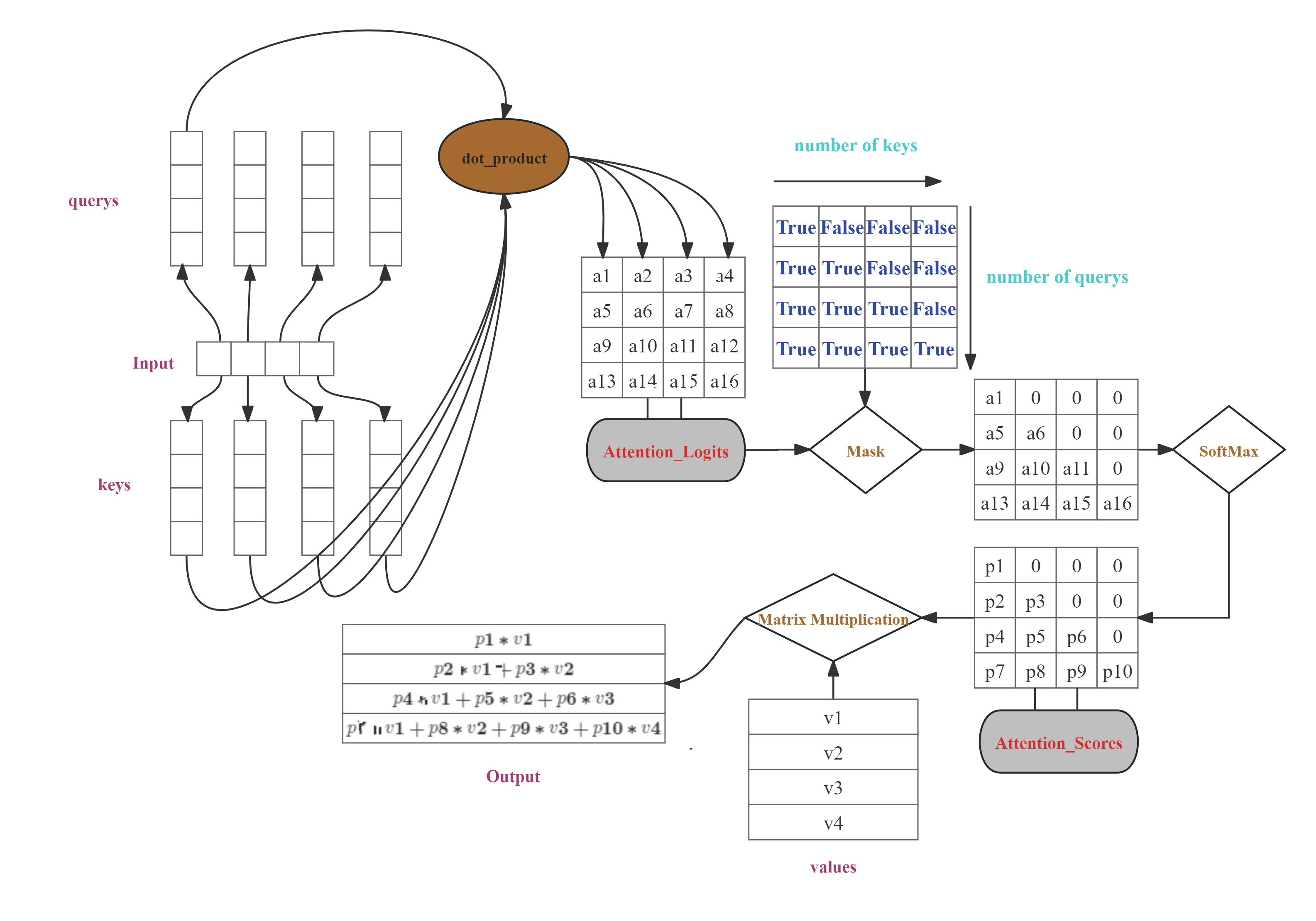
图1

Decoder和RNN一样，是串行地生成Token的。Casual Attention是带掩码的Attention——在标准的注意力分数矩阵上乘了一个下三角因果掩码矩阵，使得最终的输出具备了时序因果性——t时刻Token的预测过程不会受到t时刻之后的Key,Value以及Query的影响。因为Casual Attention这种独特掩码机制，使得Decoder在训练时可以进行并行训练，而非RNN那样只能串行训练。

2、推理阶段

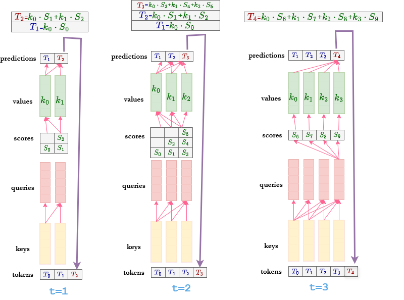
图2

Decoder在推理时是依时序串行生成Token的，这是所有Casual Attention 的作用结果。

每个Casual Atention 在推理时和训练时是一样的，t时刻上的query只会与t时刻及t时刻之前的key计算点积，t时刻上的value只会与t时刻及t时刻之前的value进行加权相加。

其中有一个关键点值得注意。如果decoder在推理时采取和训练时一样的运算流程，那么在每个时间步上，t时刻之前的value,key,query都会被重复计算。
为了提高计算效率，就有了K-V缓存技术。

3、Key-Value缓存

Key-Value缓存是运用在Decoder推理时的技术，它需要缓存每个时间步上所有Causal Attention的Key和Value。如此就可以让Decoder在下一时间步无需再计算之前的Keys和Values了，只需要得到当前的Key和Value，再将当前的Query与所有Key计算注意力分数，接着合并所有Value就行了，合并后的Value再经过预测头，就可以生产新的Token了。

Key-Value缓存能够让Decoder中所有Causal Attention在每个一时间步只需计算上一时间步预测出来的Token的Key，Value和Query。如图2，t=2时刻，2之前的Keys和Values均已缓存，只需要计算Token 的Key，Value和Query;t=3时刻，只需要计算Token 的Key，Value和Query。

每个时刻上的query是不需要缓存的，这是因为每个Casual Attention缓存了t时刻之前的value后，t时刻之前的query在t时刻就没用了，且t+1时刻的预测token只与t时刻的query以及t+1时刻之前所有value和key有关。query是有时效性的，无需缓存。

4、Casual Attention在Tensorflow中的实现原理

用Tensorflow训练一个Decoder并保存其模型结构和参数

import tensorflow as tf

# 词汇表
vocabulary_table = {1: "今", 2: "天", 3: "气", 4: "好", 5: "真"}


class Model(tf.keras.Model):
    def __init__(self, **kwargs):
        super().__init__(**kwargs)
        self.embedding = tf.keras.layers.Embedding(input_dim=6, output_dim=64, name="Embedding")
        self.casual_attention = tf.keras.layers.MultiHeadAttention(num_heads=2, key_dim=64, name="Casual_Attention")
        self.dense = tf.keras.layers.Dense(6, activation="softmax", name="output_dense")

    def call(self, inputs, training=None, mask=None):
        x = self.embedding(inputs)
        x = self.casual_attention(value=x,
                                  key=x,
                                  query=x,
                                  use_causal_mask=True)
        x = self.dense(x)
        return x

class ExportModel(tf.Module):
    def __init__(self, model):
        self.model = model

    @tf.function(input_signature=[tf.TensorSpec(shape=[1, 5], dtype=tf.float32)])
    def __call__(self, inputs):
        # training=False表明模型工作在推理模式
        result = self.model(inputs, training=False)

        return result


model = Model(name="Decoder")
# 今天天气真好
tokens = tf.constant([[1., 2., 2., 3., 5., 4.]])
Decoder_input = tokens[:, :-1]
print(Decoder_input)
Decoder_output = tokens[:, 1:]
print(Decoder_output)

model.compile(optimizer="adam", loss=tf.keras.losses.sparse_categorical_crossentropy)
model.fit(
    x=Decoder_input,
    y=Decoder_output,
    epochs=164
)
# 只保存模型参数, 模型结构需要手动构建(前向传播)
model.save_weights("Decoder_weights.h5", save_format="h5")

# 模型结构与参数全部保存
model = ExportModel(model)
tf.saved_model.save(model, "Decoder")

读取已训练好的权重参数，并手动实现Decoder的前向传播(这里的实现过程并没有使用K-V缓存)。

注意：在计算完query向量和key向量的点积后，一定要除以向量维数的平方根！

这是因为在Transformer模型中，注意力机制是核心组件。它通过query向量和key向量的点积来计算注意力分数。但当向量维度很高时，点积结果会变得非常大，这可能导致以下问题：

数值不稳定：大值在Softmax函数中会被放大，导致注意力过于集中，分布不均。

训练困难：梯度可能爆炸，影响模型稳定性。

为了解决这些问题，Transformer模型中引入了缩放注意力分数的技巧。具体来说，就是在点积后除以向量维度的平方根。这样做的好处有：
控制数值大小：将点积结果缩小到一个适中的范围，保持数值稳定。
优化Softmax表现：避免生成过于极端的概率分布，使注意力更平滑，模型学习更均匀。
训练更稳定：梯度不会因为指数函数放大而爆炸，收敛速度更快。

import tensorflow as tf
import h5py
import numpy as np


# tokens(Batch_size, num_tokens)
def forward(tokens):
    # model.save_weights()仅保存模型权重, 保存格式为.h5文件, 需要用h5py库进行读取
    # 读取模型参数文件
    weights = h5py.File("Decoder_weights.h5")

    # 打印Embedding层参数
    # (6, 64), 词汇表大小为5, 再加上一个空白词(Padding 0), 总共6个Embedding.
    embeddings_table = weights["Embedding/Decoder/Embedding/embeddings:0"][:]

    # 打印Causal Attention层参数

    # kernel : (input_dim=64, num_heads=2, key_dim=64)
    # bias : (num_heads=2, key_dim=64)
    key_dense_kernel = weights["Casual_Attention/Decoder/Casual_Attention/key/kernel:0"][:]
    key_dense_bias = weights["Casual_Attention/Decoder/Casual_Attention/key/bias:0"][:]

    # kernel : (input_dim=64, num_heads=2, query_dim=64)
    # bias : (num_heads=2, query_dim=64)
    query_dense_kernel = weights["Casual_Attention/Decoder/Casual_Attention/query/kernel:0"][:]
    query_dense_bias = weights["Casual_Attention/Decoder/Casual_Attention/query/bias:0"][:]

    # kernel : (input_dim=64, num_heads=2, value_dim=64)
    # bias : (num_heads=2, value_dim=64)
    value_dense_kernel = weights["Casual_Attention/Decoder/Casual_Attention/value/kernel:0"][:]
    value_dense_bias = weights["Casual_Attention/Decoder/Casual_Attention/value/bias:0"][:]

    # kernel : (num_heads=2, value_dim=64, output_dim=64)
    # bias : (value_dim=64,)
    attention_output_kernel = weights["Casual_Attention/Decoder/Casual_Attention/attention_output/kernel:0"][:]
    attention_output_bias = weights["Casual_Attention/Decoder/Casual_Attention/attention_output/bias:0"][:]

    # 打印最后一层密集层的参数
    # (64, 6)
    output_dense_kernel = weights["output_dense/Decoder/output_dense/kernel:0"][:]
    # (6,)
    output_dense_bias = weights["output_dense/Decoder/output_dense/bias:0"][:]

    B = tf.shape(tokens)[0]
    embeddings_table = tf.tile(embeddings_table[tf.newaxis], [B, 1, 1])
    # (Batch_size, num_tokens, embeddings_dim)
    embeddings = tf.gather_nd(embeddings_table, tokens[:, :, tf.newaxis], batch_dims=1)

    # 将embeddings分别映射成key, query, value
    key = tf.einsum("abc,cde->abde", embeddings, key_dense_kernel) + key_dense_bias
    query = tf.einsum("abc,cde->abde", embeddings, query_dense_kernel) + query_dense_bias
    value = tf.einsum("abc,cde->abde", embeddings, value_dense_kernel) + value_dense_bias

    # 计算注意力分数,

    # 计算query和key的数量积时, 一定要除以一个dim--query最后一个维度的长度
    # 因为query和key的维度很高时, 它两的数量积往往很大, 几个很大的数经过SoftMax后会产生饱和状态
    dim = tf.cast(tf.shape(query)[-1], dtype=tf.float32)

    # 生成一个下三角的掩码矩阵, 下三角是0, 上三角是一个负无穷数(-1e11)
    query_length = tf.shape(query)[1]
    key_length = tf.shape(key)[1]
    attention_mask = (1 - np.tri(N=query_length, M=key_length)) * -1e11

    # query和key的数量积矩阵加上attention_mask后,
    # 上三角全变为负无穷, 负无穷数的指数接近于0, 使得上三角的数量积在softmax中不起作用
    scores = tf.math.softmax(tf.einsum("aecd, abcd -> acbe", key, query / tf.sqrt(dim)) + attention_mask, axis=-1)

    # 利用注意力分数将value进行加权相加.
    stacked_value = tf.einsum("acbe,aecd->abcd", scores, value)

    # Causal Attention输出映射
    attention_output = tf.einsum("abcd, cde -> abe", stacked_value, attention_output_kernel) + attention_output_bias

    # 预测映射
    prediction = tf.math.softmax(tf.einsum("abc, cd -> abd", attention_output, output_dense_kernel) + output_dense_bias, axis=-1)
    return prediction


if __name__ == '__main__':
    # [1., 2., 2., 3., 5., 4.]
    tokens = tf.constant([[1, 2, 2, 3, 5]], dtype=tf.int32)
    Decoder = tf.saved_model.load("Decoder")
    print(forward(tokens)[:, -1])
    print(Decoder(tf.cast(tokens, dtype=tf.float32))[:, -1])

最后检验上述的前向传播是否实现成功，

if __name__ == '__main__':
    # [1., 2., 2., 3., 5., 4.]
    tokens = tf.constant([[1, 2, 2, 3, 5]], dtype=tf.int32)
    Decoder = tf.saved_model.load("Decoder")
    print(forward(tokens)[:, -1])
    print(Decoder(tf.cast(tokens, dtype=tf.float32))[:, -1])

最终打印结果为：

tf.Tensor(
[[1.4004541e-09 2.9884575e-10 1.6915389e-29 9.1038288e-13 9.9929798e-01
  7.0196530e-04]], shape=(1, 6), dtype=float32)
tf.Tensor(
[[1.4004541e-09 2.9884575e-10 1.6915389e-29 9.1038288e-13 9.9929798e-01
  7.0196530e-04]], shape=(1, 6), dtype=float32)

两者结果一致，且在索引4处的概率值最大，表明下一个token的预测结果为4，符合真实值。