


前言
上次发了一个二维无震源的波动方程求解。为了模拟一下地震波场的传播,这次做一个含震源的均匀介质波动方程求解。
一、控制方程、初始条件及边界条件
我们考虑在x∈[0,8];y∈[0,8]的二维空间中,存在一个沿Z轴方向振动且波速为的波场。选取雷克子波函数作为空间中的震源,则其在空间中振动时间-位移关系满足下式:
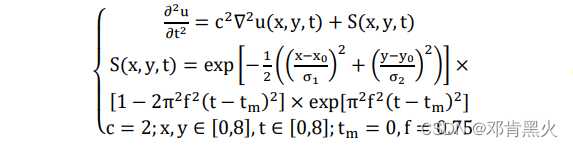
设置边界条件和初始条件如下:


二、采样点设置
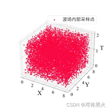
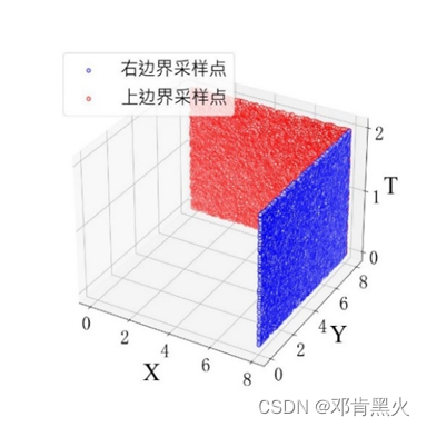
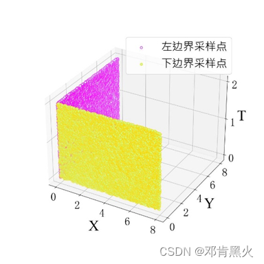
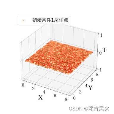
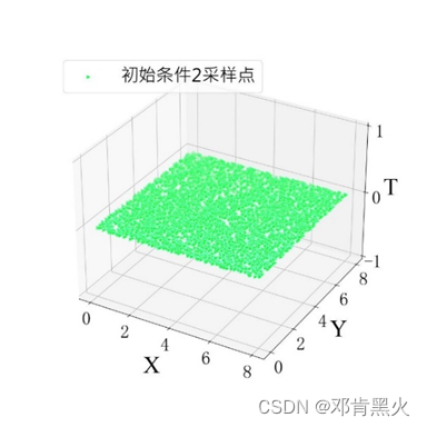
对于此二维波动方程,我们在x ∈ [0,8]; y ∈ [0,8]; t ∈ [0,2]构成的数值空间中,共计采样 10000 个采样点;在左右上下四个边界上各获取 5000 个采样点;在两个初始条件下获取 5000 个采样点。采样情况如下图所示。
三、训练
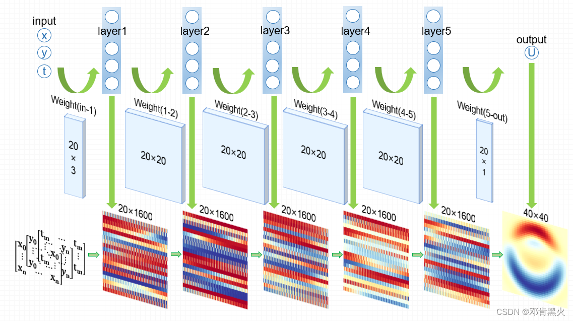
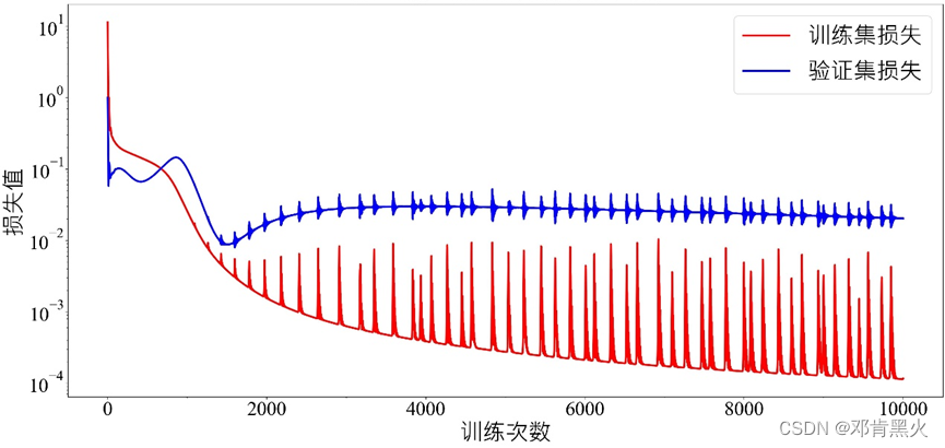
我们设置的网络主要有五个区块组成,每个区块里包含一个全连接层,以及对应的激活函数,全连接层包含 20 个节点,使用双曲正切函数为激活函数;训练期间向模型输入训练集和验证集,训练集为 3-3-2 节提到的采样数据,验证集为同样使用拉丁超立方采样算法进行采样的 1000 个波场内部采样数据;训练的学习率为0.001,预设置训练轮次为 10000 次。
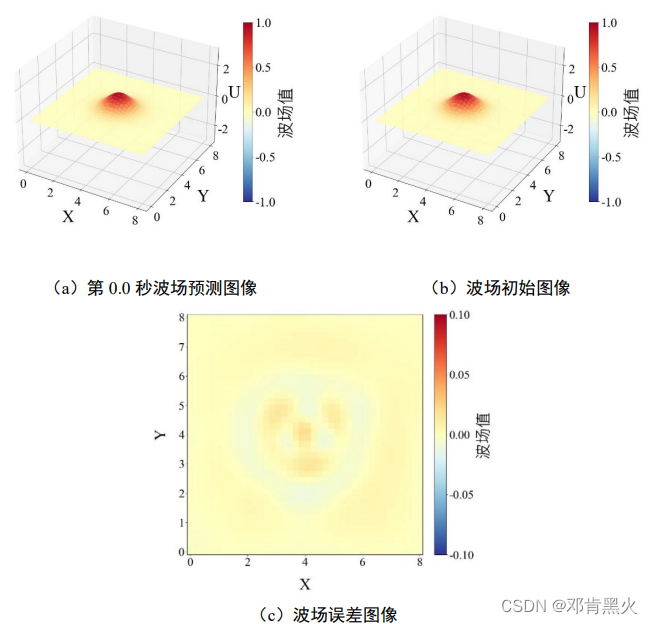
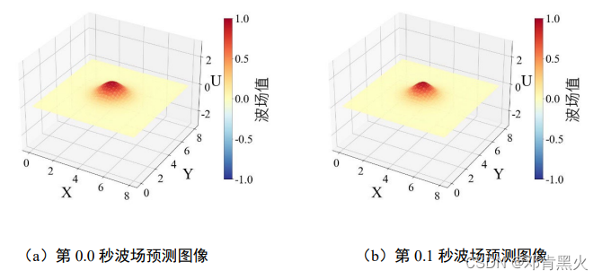
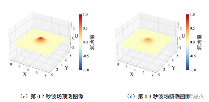
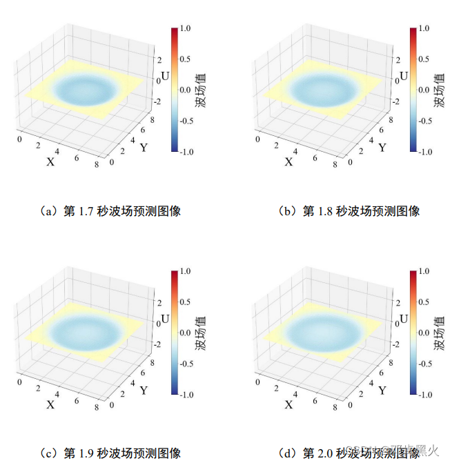
四、结果展示
先看看结果吧,反正这个东西看了也就图一乐,初始条件的拟合结果还可以,波场的传播图像也符合常识。
五、代码详解
话不多上,上代码,反正参数咱也不咋会调,只能保证跑个结果出来。
1.预前准备
######################################################################
import torch
import numpy as np
import matplotlib.pyplot as plt
from mpl_toolkits.mplot3d import Axes3D
import torch.nn as nn
from pyDOE import lhs
import imageio
import os
######################################################################
#自动更换CPU,GPU,并设置浮点型位数
default_device = "cuda" if torch.cuda.is_available() else "cpu"
dtype=torch.float32
torch.set_default_dtype(dtype)
#####################################################################
# 设置随机数种子
def setup_seed(seed):
    torch.manual_seed(seed)
    torch.cuda.manual_seed_all(seed)
    torch.backends.cudnn.deterministic = True

setup_seed(42)
######################################################################
#转换张量函数,存储损失的时候用到
def Tran_fun(tensor):
    a = []
    for i in tensor:
        i = i.to("cpu")
        i = i.detach().numpy()
        a.append(i)
    return(np.array(a))
######################################################################
#设置采样策略
def LHS_Sampling(N,be,en):
    return be + (en-be)*lhs(3, N)
######################################################################
#定义雷克子波,在激发的情况下使用
def rec_wave(x,y,t,x0,y0,t0,f):
    a = (1-2*(torch.pi*f*(t-t0))**2)*torch.exp(-(np.pi*f*(t-t0))**2)
    b = torch.exp(-0.5*((x-x0)**2+(y-y0)**2)/(0.8)**2)
    return a*b
######################################################################
#求导函数
def gradients(u, x, order=1):
    u.requires_grad_(True)
    x.requires_grad_(True)
    if order == 1:
        return torch.autograd.grad(u, x, grad_outputs=torch.ones_like(u),
                                   create_graph=True,
                                   only_inputs=True, )[0]
    else:
        return gradients(gradients(u, x), x, order=order - 1)
######################################################################
2.网络编译
######################################################################
#网络结构的编译
class PINN(nn.Module):
    def __init__(self, NN):
        super(PINN, self).__init__()

        self.input_layer = nn.Linear(3, NN)
        self.hidden_layer1 = nn.Linear(NN,NN)
        self.hidden_layer2 = nn.Linear(NN, NN)
        self.hidden_layer3 = nn.Linear(NN, NN)
        self.hidden_layer4 = nn.Linear(NN, NN)
        self.output_layer = nn.Linear(NN, 1)

    def forward(self, x): # 一种特殊的方法 __call__() 回调
        out = torch.tanh(self.input_layer(x))
        out = torch.tanh(self.hidden_layer1(out))
        out = torch.tanh(self.hidden_layer2(out))
        out = torch.tanh(self.hidden_layer3(out))
        out = torch.tanh(self.hidden_layer4(out))
        #out = torch.tanh(self.hidden_layer5(out))
        out_final = self.output_layer(out)
        return out_final

######################################################################
#损失函数,网络,优化器对象化
loss = torch.nn.MSELoss()
loss = loss.to(device = default_device)
#pinn = PINN(20)
#训练一部分保存的网络,在这里继续训练
pinn = torch.load("D:/trl/波场结构/add_resoure_wave_model2d_523.pth",map_location=torch.device('cpu'))
pinn = pinn.to(device = default_device)
opt = torch.optim.Adam(pinn.parameters(), lr=1e-3)
scheduler = torch.optim.lr_scheduler.StepLR(opt, step_size=5000, gamma=0.9)
######################################################################
3.损失函数设置
######################################################################
#pde损失函数设置
def interior_loss(Mat):
    # 内点
    Mat = torch.tensor(Mat)
    x = Mat[:, 0:1].float()
    y = Mat[:, 1:2].float()
    t = Mat[:, 2:3].float()
    x.requires_grad_(True)
    y.requires_grad_(True)
    t.requires_grad_(True)
    x = x.to(device=default_device)
    y = y.to(device = default_device)
    t = t.to(device = default_device)
    u = pinn(torch.cat([t, x, y], dim=1))
    cond1 = gradients(u, t, order=2)
    cond2 = (gradients(u, x, order=2)+gradients(u, y, order=2))*c**2 + rec_wave(x,y,t,x0=4,y0=4,t0=0,f=0.75)
    return loss(cond1,cond2)

def left_loss(Mat):
    # 左边界点
    Mat = torch.tensor(Mat)
    Mat[:,0:1] = torch.zeros_like(Mat[:,0:1])
    x = Mat[:, 0:1].float()
    y = Mat[:, 1:2].float()
    t = Mat[:, 2:3].float()
    zero = torch.zeros_like(t).float()
    x = x.to(device=default_device)
    y = y.to(device = default_device)
    t = t.to(device = default_device)
    zero = zero.to(device = default_device)
    u = pinn(torch.cat([t, x, y], dim=1))
    cond1 = u
    cond2 = zero
    return loss(cond1,cond2)

def right_loss(Mat):
    # 右边界点
    Mat = torch.tensor(Mat)
    Mat[:,0:1] = torch.ones_like(Mat[:,0:1])*8
    x = Mat[:, 0:1].float()
    y = Mat[:, 1:2].float()
    t = Mat[:, 2:3].float()
    zero = torch.zeros_like(t).float()
    x.requires_grad_(True)
    y.requires_grad_(True)
    t.requires_grad_(True)
    x = x.to(device=default_device)
    y = y.to(device = default_device)
    t = t.to(device = default_device)
    zero = zero.to(device = default_device)
    u = pinn(torch.cat([t, x, y], dim=1))
    zero = torch.zeros_like(u).requires_grad_(True)
    zero = zero.to(device = default_device)
    cond1 = u
    cond2 = zero
    return loss(cond1,cond2)

def down_loss(Mat):
    # 下边界点
    Mat = torch.tensor(Mat)
    Mat[:,1:2] = torch.zeros_like(Mat[:,1:2])
    x = Mat[:, 0:1].float()
    y = Mat[:, 1:2].float()
    t = Mat[:, 2:3].float()
    zero = torch.zeros_like(t).float()
    x.requires_grad_(True)
    y.requires_grad_(True)
    t.requires_grad_(True)
    zero.requires_grad_(True)
    x = x.to(device=default_device)
    y = y.to(device = default_device)
    t = t.to(device = default_device)
    zero = zero.to(device = default_device)
    u = pinn(torch.cat([t, x, y], dim=1))
    cond1 = u
    cond2 = zero
    return loss(cond1,cond2)

def up_loss(Mat):
    # 上边界点
    Mat = torch.tensor(Mat)
    Mat[:,1:2] = torch.ones_like(Mat[:,1:2])*8
    x = Mat[:, 0:1].float()
    y = Mat[:, 1:2].float()
    t = Mat[:, 2:3].float()
    zero = torch.zeros_like(t).float()
    x.requires_grad_(True)
    y.requires_grad_(True)
    t.requires_grad_(True)
    x = x.to(device=default_device)
    y = y.to(device = default_device)
    t = t.to(device = default_device)
    zero = zero.to(device = default_device)
    u = pinn(torch.cat([t, x, y], dim=1))
    cond1 = u
    cond2 = zero
    return loss(cond1,cond2)

def ini1_loss(Mat):
    # 初始条件1
    Mat = torch.tensor(Mat)
    Mat[:,2:3] = torch.zeros_like(Mat[:,2:3])
    x = Mat[:, 0:1].float()
    y = Mat[:, 1:2].float()
    t = Mat[:, 2:3].float()
    zero = torch.zeros_like(t).float()
    x.requires_grad_(True)
    y.requires_grad_(True)
    t.requires_grad_(True)
    zero.requires_grad_(True)
    x = x.to(device=default_device)
    y = y.to(device = default_device)
    t = t.to(device = default_device)
    u = pinn(torch.cat([t, x, y], dim=1))
    cond1 = u
    cond2 = rec_wave(x,y,t,x0=4,y0=4,t0=0,f=0.75)
    return loss(cond1,cond2)

def ini2_loss(Mat):
    # 初始条件2
    Mat = torch.tensor(Mat)
    Mat[:,2:3] = torch.zeros_like(Mat[:,2:3])
    x = Mat[:, 0:1].float()
    y = Mat[:, 1:2].float()
    t = Mat[:, 2:3].float()
    zero = torch.zeros_like(t).float()
    x.requires_grad_(True)
    y.requires_grad_(True)
    t.requires_grad_(True)
    zero.requires_grad_(True)
    x = x.to(device=default_device)
    y = y.to(device = default_device)
    t = t.to(device = default_device)
    u = pinn(torch.cat([t, x, y], dim=1))
    cond1 = gradients(u, t, order=1)
    cond2 = torch.exp(-0.5*((x-4)**2+(y-4)**2)/(0.8)**2)
    return loss(cond1,cond2)
######################################################################
4.网络训练
#####################################################################
#参数设置
c,len_x,len_y,len_t = 2, 2, 2,6
t_b,t_e,t_num = 0.0,2,21
x_b,x_e,x_num = 0.0,8,40
y_b,y_e,y_num = 0.0,8,40
sample_num = 10000
######################################################################
#范围设置
t_range = [t_b, t_e]
x_range = [x_b, x_e]
y_range = [y_b, y_e]
lb = np.asarray([x_range[0], y_range[0], t_range[0]])
ub = np.asarray([x_range[1], y_range[1], t_range[1]])
#内点,边界,初始条件采样
xyt_in = LHS_Sampling(sample_num,lb,ub)
xyt_left = LHS_Sampling(sample_num,lb,ub)
xyt_right = LHS_Sampling(sample_num,lb,ub)
xyt_down = LHS_Sampling(sample_num,lb,ub)
xyt_up = LHS_Sampling(sample_num,lb,ub)
xyt_ini1 = LHS_Sampling(sample_num,lb,ub)
xyt_ini2 = LHS_Sampling(sample_num,lb,ub)
######################################################################
######################################################################
#设置训练次数,设置接收损失值的列表
epochs = 10000
loss_i,loss_le,loss_ri,loss_d,loss_u,loss_i1,loss_i2,loss_all = [],[],[],[],[],[],[],[]
######################################################################
#训练
for i in range(epochs):
    opt.zero_grad()
    a1= interior_loss(xyt_in)
    a2 = left_loss(xyt_left)
    a3 = right_loss(xyt_right)
    a4 = down_loss(xyt_down)
    a5 = up_loss(xyt_up)
    a6 = ini1_loss(xyt_ini1)
    a7 = ini2_loss(xyt_ini2)
    l = a1+a2+a3+a4+a5+a6+a6
    loss_all.append(l)
    l.backward()
    opt.step()
    if i % 100 == 0:
        print(i,l)
c8 = Tran_fun(loss_all)
5.网络保存
##################################################################
model = pinn
#torch.save(pinn,"D:/trl/波场结构/add_resoure_wave_model2d.pth")
##################################################################
6.绘图函数编写
这里给了两个绘图函数,可以画平面图,可以画3D图
######################################################################
#编写绘图
class Output_Fun():
    def __init__(self, t_b,t_e,t_num,x_b,x_e,x_num,y_b,y_e,y_num):
        self.t_b = t_b
        self.t_e = t_e
        self.t_num = t_num
        self.x_b = x_b
        self.x_e = x_e
        self.x_num = x_num
        self.y_b = y_b
        self.y_e = y_e
        self.y_num = y_num

    def U_Pred(self,model_path):
        model = torch.load(model_path,map_location=torch.device('cpu'))
        tc = torch.linspace(self.t_b, self.t_e, self.t_num)
        xc = torch.linspace(self.x_b, self.x_e, self.x_num)
        yc = torch.linspace(self.y_b, self.y_e, self.y_num)
        tm, xm, ym = torch.meshgrid(tc, xc, yc)
        xx = xm.reshape(-1, 1)
        yy = ym.reshape(-1, 1)
        tt = tm.reshape(-1, 1)
        xy = torch.cat([tt,xx,yy], dim=1)
        u_pred = model(xy)
        return u_pred

    def U_Draw(self,pred_mat):
        plt.rcParams['font.sans-serif']=["Times New Roman"] # 用来正常显示中文标签
        plt.rcParams['axes.unicode_minus']=False # 用来正常显示
        my_font_label = {"family":"Microsoft JhengHei", "size":40}
        my_font_title = {"family":"Microsoft JhengHei", "size":50}
        my_font_ax = {"family":"Times New Roman", "size":40}
        x = torch.linspace(self.x_b,self.x_e,self.x_num)
        y = torch.linspace(self.y_b,self.y_e,self.y_num)
        X,Y = torch.meshgrid(x,y)
        dt = (self.t_e-self.t_b)/int(self.t_num-1)
        pred_mat = pred_mat.detach().numpy()
        lenspace = int(self.x_num**2)
        frames_pre = []
        for i in range(0,int(self.t_num),1):
            u_i = pred_mat[i*lenspace:(i+1)*lenspace,:].reshape((self.x_num,self.y_num))
            fig = plt.figure(figsize=(10,10),tight_layout=True)
            t = round(dt*i,3)

            ax = fig.add_subplot(111,projection='3d')
            ax.set_zlim3d(zmin=-3, zmax=3)
            ax.set_xlabel('X',fontdict=my_font_ax,labelpad=25)
            ax.set_ylabel('Y',fontdict=my_font_ax,labelpad=25)
            ax.set_zlabel('U',fontdict=my_font_ax,labelpad=5)
            #ax.set_title("第"+str(t)+"秒波场预测图像",fontdict=my_font_title)
            ax.tick_params(labelsize=30)

            surf = ax.plot_trisurf(X.reshape(-1), Y.reshape(-1), u_i.reshape(-1),cmap='RdYlBu_r',vmin =-1,vmax=1)
            cb=fig.colorbar(surf,shrink=0.6,aspect=20,ticks=np.linspace(-1,1,5))
            cb.ax.tick_params(labelsize=30)  #设置色标刻度字体大小。
            cb.set_label('波场值',fontdict=my_font_label) #设置colorbar的标签字体及其大小


            plt.savefig("D:/trl/图像波场/含震源二维预测波场/第"+str(t)+"秒波场图像.jpg")
            #image_name = "D:/trl/图像波场/含震源二维预测波场/第"+str(t)+"秒波场图像.jpg"
            #frames_pre.append(imageio.imread(image_name))
        #imageio.mimsave("D:/trl/图像波场/含震源二维预测波场/pred.gif", frames_pre, 'GIF', duration=0.2) # 保存在当前文件夹
######################################################################
#编写绘图
class Output_Fun_plane():
    def __init__(self, t_b,t_e,t_num,x_b,x_e,x_num,y_b,y_e,y_num):
        self.t_b = t_b
        self.t_e = t_e
        self.t_num = t_num
        self.x_b = x_b
        self.x_e = x_e
        self.x_num = x_num
        self.y_b = y_b
        self.y_e = y_e
        self.y_num = y_num

    def U_Pred(self,model_path):
        model = torch.load(model_path,map_location=torch.device('cpu'))
        tc = torch.linspace(self.t_b, self.t_e, self.t_num)
        xc = torch.linspace(self.x_b, self.x_e, self.x_num)
        yc = torch.linspace(self.y_b, self.y_e, self.y_num)
        tm, xm, ym = torch.meshgrid(tc, xc, yc)
        xx = xm.reshape(-1, 1)
        yy = ym.reshape(-1, 1)
        tt = tm.reshape(-1, 1)
        xy = torch.cat([tt,xx,yy], dim=1)
        u_pred = model(xy)
        return u_pred

    def U_Draw(self,pred_mat):
        plt.rcParams['font.sans-serif']=['Times New Roman'] # 用来正常显示中文标签
        plt.rcParams['axes.unicode_minus']=False # 用来正常显示
        my_font_label = {"family":"Microsoft JhengHei", "size":40}
        my_font_title = {"family":"Microsoft JhengHei", "size":50}
        my_font_ax = {"family":"Times New Roman", "size":40}
        x = torch.linspace(self.x_b,self.x_e,self.x_num)
        y = torch.linspace(self.y_b,self.y_e,self.y_num)
        X,Y = torch.meshgrid(x,y)
        dt = (self.t_e-self.t_b)/int(self.t_num-1)
        pred_mat = pred_mat.detach().numpy()
        lenspace = int(self.x_num**2)
        frames_pre = []
        for i in range(0,int(self.t_num),1):
            u_i = pred_mat[i*lenspace:(i+1)*lenspace,:].reshape((self.x_num,self.y_num))
            fig = plt.figure(figsize=(12,10))
            t = round(dt*i,3)

            ax = fig.add_subplot(111)
            ax.set_xlabel('X',fontdict=my_font_ax,labelpad=25)
            ax.set_ylabel('Y',fontdict=my_font_ax,labelpad=25)
            ax.set_title("第"+str(t)+"秒波场预测图像",fontdict=my_font_title)
            ax.tick_params(labelsize=30)

            surf = ax.pcolor(X, Y, u_i,cmap='RdYlBu_r',vmin =-0.3,vmax=0.3)
            cb=fig.colorbar(surf,shrink=1,aspect=20,ticks=np.linspace(-0.3,0.3,7))
            cb.ax.tick_params(labelsize=30)  #设置色标刻度字体大小。
            cb.set_label('波场值',fontdict=my_font_label) #设置colorbar的标签字体及其大小


            plt.savefig("D:/trl/图像波场/含震源二维预测波场/第"+str(t)+"秒波场图像二维.jpg")
5.网络保存
#求解方程并绘制3D图像
t_b,t_e,t_num = 0.0,2,21
x_b,x_e,x_num = 0.0,8,40
y_b,y_e,y_num = 0.0,8,40
sol = Output_Fun(t_b,t_e,t_num,x_b,x_e,x_num,y_b,y_e,y_num)
mat1 = sol.U_Pred("D:/trl/波场结构/add_resoure_wave_model2d.pth")
sol.U_Draw(mat1)
######################################################################
#求解方程并绘制图像
#sol = Output_Fun_plane(t_b,t_e,t_num,x_b,x_e,x_num,y_b,y_e,y_num)
#mat1 = sol.U_Pred("D:/trl/波场结构/add_resoure_wave_model2d.pth")
#sol.U_Draw(mat1)
######################################################################
最后的话
这是一个均匀层状介质模型的实现,但是我一直没有调到非常满意的结果,可以看看这两张gif图片,效果就是这样。下一期会给出一个层状介质的模拟结果,也是这个系列的最后一期了。


 873
873

 被折叠的 条评论
为什么被折叠?
被折叠的 条评论
为什么被折叠?
 到【灌水乐园】发言


