


目录
1.3 Feedforward and cost function
2.5 Regularized Neural Networks
2.6 Learning parameters using fmincg
1. Neural Networks
内容:我们将使用反向传播来学习神经网络所需的参数(权重)。
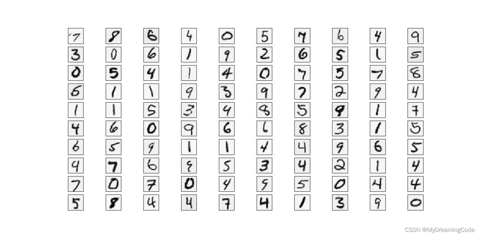
1.1 Visualizing the data
内容:一共有5000个训练集,X为5000×400维度,每行样本数据表示一个由20×20像素组成的手写数字识别图像。y为每个样本的真实标签(注意:0对应的标签为10),维度为5000×1。
main.py
from scipy.io import loadmat  # 导入MATLAB格式数据

data = loadmat('ex4data.mat')
X, y = data['X'], data['y']
weights = loadmat('ex4weights.mat')
Theta1, Theta2 = weights['Theta1'], weights['Theta2']

print(X.shape, y.shape, Theta1.shape, Theta2.shape)
# (5000, 400) (5000, 1) (25, 401) (10, 26)
plot.py
import numpy as np
import matplotlib.pyplot as plt
import matplotlib

def Plot(X):
    sample_idx = np.random.choice(np.arange(X.shape[0]), 100)  # 从0-4999中随机抽取100个数
    sample_image = X[sample_idx, :]
    fig, axisArr = plt.subplots(nrows=10, ncols=10, sharex=True, sharey=True, figsize=(10, 10))
    for r in range(10):
        for c in range(10):
            axisArr[r, c].matshow(sample_image[r * 10 + c].reshape(20, 20).T, cmap=matplotlib.cm.binary)
    plt.xticks(np.array([]))
    plt.yticks(np.array([]))
    plt.show()
main.py
from scipy.io import loadmat  # 导入MATLAB格式数据
from plot import *  # 绘图

data = loadmat('ex4data.mat')
X, y = data['X'], data['y']
weights = loadmat('ex4weights.mat')
Theta1, Theta2 = weights['Theta1'], weights['Theta2']
Plot(X)
1.2 Model representation
内容:Theta1:25×401 Theta2:10 ×26

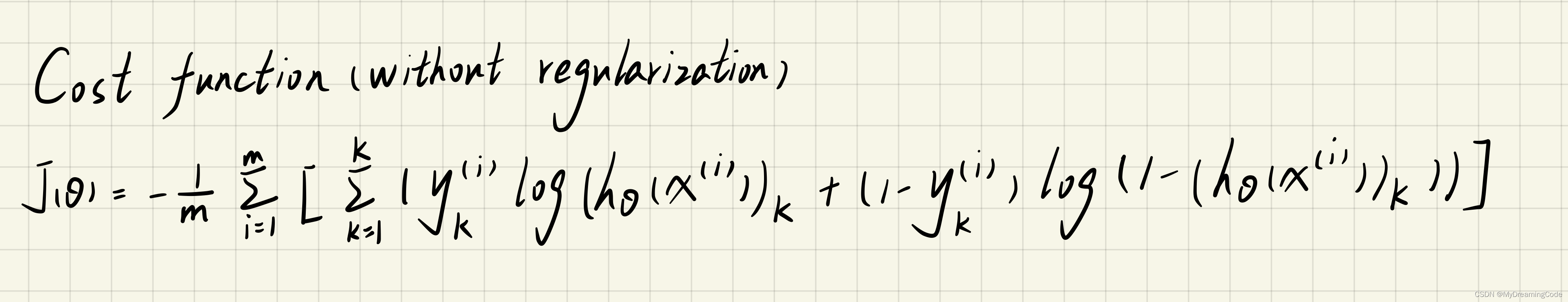
1.3 Feedforward and cost function
内容:根据已给出的Theta1和Theta2进行前向传播以及计算代价函数。特别注意,这里真实标签y需要重新编码一下,可更新为5000×10维度的矩阵,用于计算代价函数。
sigmoid.py
import numpy as np

def Sigmoid(z):
    return 1 / (1 + np.exp(-z))
forward_propagate.py
import numpy as np
from sigmoid import *

def forwardPropagate(Theta1, Theta2, X):
    X = np.insert(X, 0, values=np.ones(X.shape[0]), axis=1)
    a1 = X
    z2 = a1 * Theta1.T
    a2 = Sigmoid(z2)
    a2 = np.insert(a2, 0, values=np.ones(a2.shape[0]), axis=1)
    z3 = a2 * Theta2.T
    h_theta = Sigmoid(z3)
    return h_theta
cost_function.py
import numpy as np
from sklearn.preprocessing import OneHotEncoder  # 数据预处理
from forward_propagate import *  # 前向传播

def costFunction(Theta1, Theta2, X, y):
    X = np.matrix(X)
    Theta1 = np.matrix(Theta1)
    Theta2 = np.matrix(Theta2)
    m = X.shape[0]
    h_theta = forwardPropagate(Theta1, Theta2, X)
    # 对y标签进行编码,使其变成5000×10维度的矩阵
    encoder = OneHotEncoder(sparse=False)
    y_onehot = encoder.fit_transform(y)
    # print(y[0], y_onehot[0, :])  # [10] [0. 0. 0. 0. 0. 0. 0. 0. 0. 1.]
    first = np.sum(np.multiply(y_onehot, np.log(h_theta)), axis=1)
    second = np.sum(np.multiply(1 - y_onehot, np.log(1 - h_theta)), axis=1)
    J_theta = -np.sum(first + second) / m
    return J_theta
main.py
from scipy.io import loadmat  # 导入MATLAB格式数据
from plot import *  # 绘图
from cost_function import *  # 代价函数

data = loadmat('ex4data.mat')
X, y = data['X'], data['y']
weights = loadmat('ex4weights.mat')
Theta1, Theta2 = weights['Theta1'], weights['Theta2']
print(costFunction(Theta1, Theta2, X, y))
0.2876291651613189
1.4 Regularized cost function
内容:将代价函数进行正则化
cost_function_reg.py
import numpy as np
from sklearn.preprocessing import OneHotEncoder  # 数据预处理
from forward_propagate import *  # 前向传播

def costFunctionReg(Theta1, Theta2, X, y, learningRate):
    X = np.matrix(X)
    Theta1 = np.matrix(Theta1)
    Theta2 = np.matrix(Theta2)
    m = X.shape[0]
    h_theta = forwardPropagate(Theta1, Theta2, X)
    # 对y标签进行编码,使其变成5000×10维度的矩阵
    encoder = OneHotEncoder(sparse=False)
    y_onehot = encoder.fit_transform(y)
    first = np.sum(np.multiply(y_onehot, np.log(h_theta)), axis=1)
    second = np.sum(np.multiply(1 - y_onehot, np.log(1 - h_theta)), axis=1)
    reg = np.sum(np.power(Theta1[:, 1:], 2)) + np.sum(np.power(Theta2[:, 1:], 2))
    J_theta = -np.sum(first + second) / m + learningRate * reg / (2 * m)
    return J_theta
main.py
from scipy.io import loadmat  # 导入MATLAB格式数据
from plot import *  # 绘图
from cost_function_reg import *  # 代价函数

data = loadmat('ex4data.mat')
X, y = data['X'], data['y']
weights = loadmat('ex4weights.mat')
Theta1, Theta2 = weights['Theta1'], weights['Theta2']
learningRate = 1
print(costFunctionReg(Theta1, Theta2, X, y, learningRate))
0.38376985909092365
2. Backpropagation
内容:利用反向传播来计算神经网络代价函数的梯度,从而将代价函数值最小化。
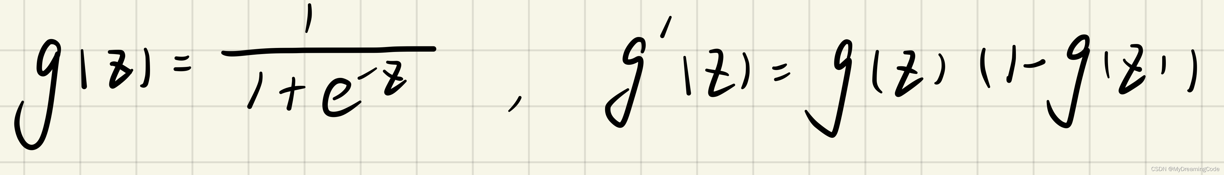
2.1 Sigmoid gradient
sigmoid_gradient.py
import numpy as np
from sigmoid import *

def sigmoidGradient(z):
    return np.multiply(Sigmoid(z), 1 - Sigmoid(z))

# print(sigmoidGradient(0))  # 0.25
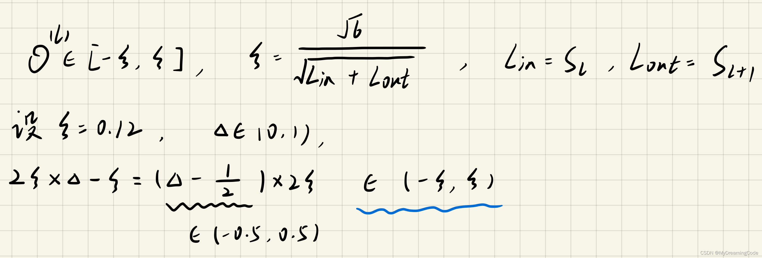
2.2 Random initialization
内容:初始化theta的值。Lin为l层的单元数,Lout为l+1层的单元数。
main.py
from scipy.io import loadmat  # 导入MATLAB格式数据
from plot import *  # 绘图
from cost_function_reg import *  # 代价函数
import numpy as np

data = loadmat('ex4data.mat')
X, y = data['X'], data['y']
weights = loadmat('ex4weights.mat')
Theta1, Theta2 = weights['Theta1'], weights['Theta2']
# 初始化值
learningRate = 1
input_size = 400
hidden_size = 25
num_labels = 10
# np.random.random(size):size指所生成随机数0-1的维度大小
# 这里设范围为[-0.12,0.12]
params = (np.random.random(size=hidden_size * (input_size + 1) + num_labels * (hidden_size + 1)) - 0.5) * 2 * 0.12
# print(params)
# [-0.09845394  0.07595105  0.05357422 ... -0.11991807 -0.08736149
#  -0.09793505]
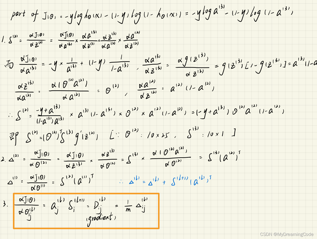
2.3 Backpropagation
内容: 求误差项,误差项用于衡量此节点对于最后的输出误差的贡献度。
a. 正向传播

b. 反向传播
forward_propagate.py(增加了返回项)
import numpy as np
from sigmoid import *

def forwardPropagate(Theta1, Theta2, X):
    X = np.insert(X, 0, values=np.ones(X.shape[0]), axis=1)
    a1 = X
    z2 = a1 * Theta1.T
    a2 = Sigmoid(z2)
    a2 = np.insert(a2, 0, values=np.ones(a2.shape[0]), axis=1)
    z3 = a2 * Theta2.T
    h_theta = Sigmoid(z3)
    return a1, z2, a2, z3, h_theta
注意:
1. 在计算误差项时,Z2需要变成26×1(维度)
2. 在训练集上算整体的误差项,所以要在for循环中使用delta_l=delta_l+..
back_propagation.py
import numpy as np
from forward_propagate import *  # 正向传播
from sigmoid_gradient import *  # 激活函数的导数

def backPropagation(params, input_size, hidden_size, num_labels, X, y):
    X = np.matrix(X)
    y = np.matrix(y)
    m = X.shape[0]
    Theta1 = np.matrix(np.reshape(params[:hidden_size * (input_size + 1)], (hidden_size, input_size + 1)))
    Theta2 = np.matrix(np.reshape(params[hidden_size * (input_size + 1):], (num_labels, hidden_size + 1)))
    # 1. feedforward->z、a、h
    a1, z2, a2, z3, h_theta = forwardPropagate(Theta1, Theta2, X)
    # print(a1.shape, z2.shape, a2.shape, h_theta.shape)
    # (5000, 401) (5000, 25) (5000, 26) (5000, 10)
    # 1.初始化梯度以及代价函数
    J = 0
    delta1 = np.zeros(Theta1.shape)
    delta2 = np.zeros(Theta2.shape)
    # print(delta1.shape, delta2.shape)  # (25, 401) (10, 26)
    # 2.计算代价函数
    first_term = np.sum(np.multiply(y, np.log(h_theta)))
    second_term = np.sum(np.multiply(1 - y, np.log(1 - h_theta)))
    J = -(first_term + second_term) / m
    # 3.反向传播计算出误差项(在训练集上算整体的误差项,故要用delta=delta+..)、梯度
    for i in range(m):
        a1i = a1[i, :]  # (1,401)
        z2i = z2[i, :]  # (1,25)
        a2i = a2[i, :]  # (1,26)
        h_thetai = h_theta[i, :]  # (1,10)
        yi = y[i, :]  # (1,10)

        d_error3 = h_thetai - yi  # (1,10)
        # 将z2的维度变成26×1
        z2i = np.insert(z2i, 0, values=np.ones(1))  # (1,26)
        # 求隐藏层的误差项
        d_error2 = np.multiply((Theta2.T * d_error3.T).T, sigmoidGradient(z2i))  # (1,26)
        # 求整个训练集的梯度delta1与delta2
        delta1 = delta1 + (d_error2[:, 1:]).T * a1i
        delta2 = delta2 + d_error3.T * a2i
    delta1 = delta1 / m
    delta2 = delta2 / m
    return J, delta1, delta2
main.py
from scipy.io import loadmat  # 导入MATLAB格式数据
import numpy as np
from sklearn.preprocessing import OneHotEncoder  # 数据预处理
from back_propagation import *  # 反向传播

data = loadmat('ex4data.mat')
X, y = data['X'], data['y']
weights = loadmat('ex4weights.mat')
Theta1, Theta2 = weights['Theta1'], weights['Theta2']
# 初始化值
input_size = 400
hidden_size = 25
num_labels = 10
params = (np.random.random(size=hidden_size * (input_size + 1) + num_labels * (hidden_size + 1)) - 0.5) * 2 * 0.12
encoder = OneHotEncoder(sparse=False)
y_onehot = encoder.fit_transform(y)
backPropagation(params, input_size, hidden_size, num_labels, X, y_onehot)
2.4 Gradient Checking
内容:用于检查梯度是否正确。

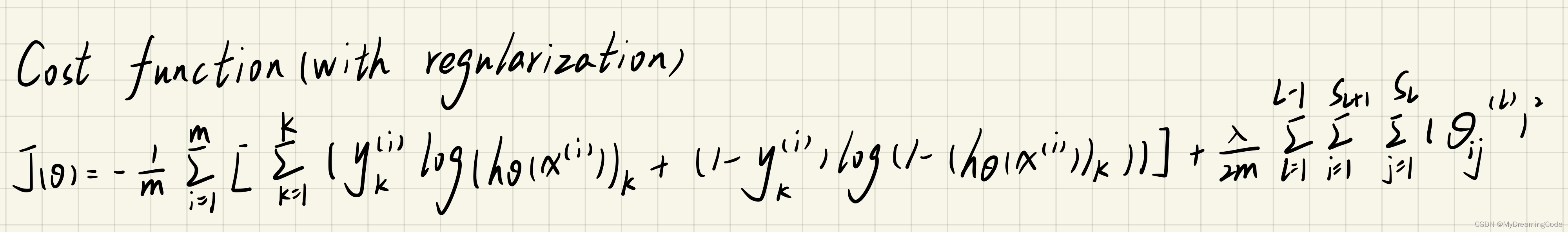
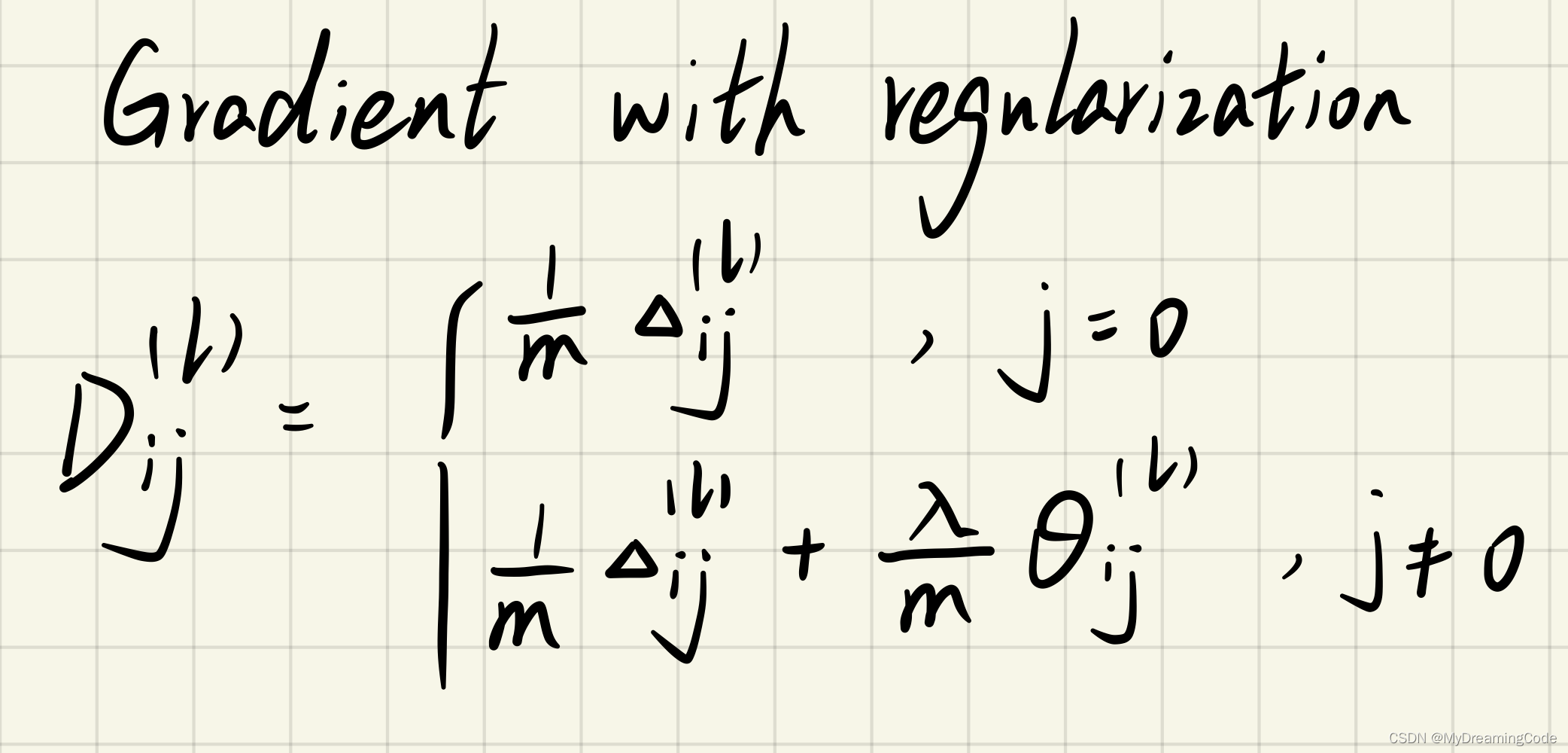
2.5 Regularized Neural Networks
内容:正则化神经网络,即在之前的式子中加入正则项。
注意:用于偏置项的那一列不需要正则化。
back_propagation_reg.py
import numpy as np
from forward_propagate import *  # 正向传播
from sigmoid_gradient import *  # 激活函数的导数

def backPropagationReg(params, input_size, hidden_size, num_labels, X, y, learningRate):
    X = np.matrix(X)
    y = np.matrix(y)
    m = X.shape[0]
    Theta1 = np.matrix(np.reshape(params[:hidden_size * (input_size + 1)], (hidden_size, input_size + 1)))
    Theta2 = np.matrix(np.reshape(params[hidden_size * (input_size + 1):], (num_labels, hidden_size + 1)))
    # 1. feedforward->z、a、h
    a1, z2, a2, z3, h_theta = forwardPropagate(Theta1, Theta2, X)
    # print(a1.shape, z2.shape, a2.shape, h_theta.shape)
    # (5000, 401) (5000, 25) (5000, 26) (5000, 10)
    # 1.初始化梯度以及代价函数
    J = 0
    delta1 = np.zeros(Theta1.shape)
    delta2 = np.zeros(Theta2.shape)
    # print(delta1.shape, delta2.shape)  # (25, 401) (10, 26)
    # 2.计算代价函数
    first_term = np.sum(np.multiply(y, np.log(h_theta)))
    second_term = np.sum(np.multiply(1 - y, np.log(1 - h_theta)))
    J = -(first_term + second_term) / m
    # 3.反向传播计算出误差项(在训练集上算整体的误差项,故要用delta=delta+..)、梯度
    for i in range(m):
        a1i = a1[i, :]  # (1,401)
        z2i = z2[i, :]  # (1,25)
        a2i = a2[i, :]  # (1,26)
        h_thetai = h_theta[i, :]  # (1,10)
        yi = y[i, :]  # (1,10)

        d_error3 = h_thetai - yi  # (1,10)
        # 将z2的维度变成26×1
        z2i = np.insert(z2i, 0, values=np.ones(1))  # (1,26)
        # 求隐藏层的误差项
        d_error2 = np.multiply((Theta2.T * d_error3.T).T, sigmoidGradient(z2i))  # (1,26)
        # 求整个训练集的梯度delta1与delta2
        delta1 = delta1 + (d_error2[:, 1:]).T * a1i
        delta2 = delta2 + d_error3.T * a2i
    delta1 = delta1 / m
    delta2 = delta2 / m
    # 3.添加正则项(用于偏置项的那一列不需要正则化)
    delta1[:, 1:] = delta1[:, 1:] + (learningRate * Theta1[:, 1:]) / m
    delta2[:, 1:] = delta2[:, 1:] + (learningRate * Theta2[:, 1:]) / m
    # np.ravel:用于将多维数组变成一维数组
    # np.concatenate((a,b)):用于将多个数组拼接
    grad = np.concatenate((np.ravel(delta1), np.ravel(delta2)))
    return J, grad
main.py
from scipy.io import loadmat  # 导入MATLAB格式数据
import numpy as np
from sklearn.preprocessing import OneHotEncoder  # 数据预处理
from back_propagation_reg import *  # 反向传播

data = loadmat('ex4data.mat')
X, y = data['X'], data['y']
weights = loadmat('ex4weights.mat')
Theta1, Theta2 = weights['Theta1'], weights['Theta2']
# 初始化值
input_size = 400
hidden_size = 25
num_labels = 10
learningRate = 1
params = (np.random.random(size=hidden_size * (input_size + 1) + num_labels * (hidden_size + 1)) - 0.5) * 2 * 0.12
encoder = OneHotEncoder(sparse=False)
y_onehot = encoder.fit_transform(y)
backPropagationReg(params, input_size, hidden_size, num_labels, X, y_onehot, learningRate)
2.6 Learning parameters using fmincg
内容:使用fmincg得到参数最优解。
from scipy.io import loadmat  # 导入MATLAB格式数据
import numpy as np
from sklearn.preprocessing import OneHotEncoder  # 数据预处理
from scipy.optimize import minimize  # 提供最优化算法函数
from back_propagation_reg import *  # 反向传播

data = loadmat('ex4data.mat')
X, y = data['X'], data['y']
weights = loadmat('ex4weights.mat')
Theta1, Theta2 = weights['Theta1'], weights['Theta2']
# 初始化值
input_size = 400
hidden_size = 25
num_labels = 10
learningRate = 1
params = (np.random.random(size=hidden_size * (input_size + 1) + num_labels * (hidden_size + 1)) - 0.5) * 2 * 0.12
encoder = OneHotEncoder(sparse=False)
y_onehot = encoder.fit_transform(y)
backPropagationReg(params, input_size, hidden_size, num_labels, X, y_onehot, learningRate)
# 1.fun:目标函数
# 2.x0:初始的猜测
# 3.args=():优化的附加参数
# 4.method:要使用的方法名称,这里使用的TNC(截断牛顿算法)
# 5.jac=True,则假定fun会返回梯度以及目标函数,若为False,则将以数字方式估计梯度
# 6.options={..},带字典类型进去,maxiter指最大迭代次数
fmin = minimize(fun=backPropagationReg, x0=params,
                args=(input_size, hidden_size, num_labels, X, y_onehot, learningRate), method='TNC', jac=True,
                options={'maxiter': 250})
print(fmin)  # x-解决方案
message: Max. number of function evaluations reached
success: False
status: 3
fun: 0.1509371037493068
x: [ 1.432e-01 -5.233e-03 ... -5.369e-01 -2.709e-01]
nit: 22
jac: [ 1.612e-04 -1.047e-06 ... -9.244e-05 -9.776e-05]
nfev: 250
用优化后的参数来进行预测(精确度可达98%):
main.py
from scipy.io import loadmat  # 导入MATLAB格式数据
import numpy as np
from sklearn.preprocessing import OneHotEncoder  # 数据预处理
from sklearn.metrics import classification_report  # 常用的输出模型评估报告方法
from scipy.optimize import minimize  # 提供最优化算法函数
from back_propagation_reg import *  # 反向传播
from forward_propagate import *  # 前向传播

data = loadmat('ex4data.mat')
X, y = data['X'], data['y']
weights = loadmat('ex4weights.mat')
Theta1, Theta2 = weights['Theta1'], weights['Theta2']
# 初始化值
input_size = 400
hidden_size = 25
num_labels = 10
learningRate = 1
params = (np.random.random(size=hidden_size * (input_size + 1) + num_labels * (hidden_size + 1)) - 0.5) * 2 * 0.12
encoder = OneHotEncoder(sparse=False)
y_onehot = encoder.fit_transform(y)
backPropagationReg(params, input_size, hidden_size, num_labels, X, y_onehot, learningRate)
fmin = minimize(fun=backPropagationReg, x0=params,
                args=(input_size, hidden_size, num_labels, X, y_onehot, learningRate), method='TNC', jac=True,
                options={'maxiter': 250})
X = np.matrix(X)
thetafinal1 = np.matrix(np.reshape(fmin.x[:(input_size + 1) * hidden_size], (hidden_size, input_size + 1)))
thetafinal2 = np.matrix(np.reshape(fmin.x[(input_size + 1) * hidden_size:], (num_labels, hidden_size + 1)))
a1, z2, a2, z3, h_theta = forwardPropagate(thetafinal1, thetafinal2, X)
# 对于argmax,axis=1,是在行中比较,选出最大的列索引
y_pred = np.array(np.argmax(h_theta, axis=1) + 1)
print(classification_report(y, y_pred))
# precision recall f1-score support
# 精确率     召回率  调和平均数  支持度(指原始的真实数据中属于该类的个数)
precision recall f1-score support
1 0.98 0.99 0.99 500
2 0.99 0.98 0.99 500
3 0.99 0.98 0.98 500
4 0.99 0.99 0.99 500
5 0.99 0.99 0.99 500
6 0.99 0.99 0.99 500
7 0.99 0.99 0.99 500
8 0.99 1.00 1.00 500
9 0.99 0.98 0.98 500
10 0.99 1.00 0.99 500accuracy 0.99 5000
macro avg 0.99 0.99 0.99 5000
weighted avg 0.99 0.99 0.99 5000
3. Visualizing the hidden layer
内容:将隐藏层(25个单元)所表达的东西可视化出来。
plot.py
import numpy as np
import matplotlib.pyplot as plt
import matplotlib

def Plot(X):
    sample_idx = np.random.choice(np.arange(X.shape[0]), 100)  # 从0-4999中随机抽取100个数
    sample_image = X[sample_idx, :]
    fig, axisArr = plt.subplots(nrows=10, ncols=10, sharex=True, sharey=True, figsize=(10, 10))
    for r in range(10):
        for c in range(10):
            axisArr[r, c].matshow(sample_image[r * 10 + c].reshape(20, 20).T, cmap=matplotlib.cm.binary)
    plt.xticks(np.array([]))
    plt.yticks(np.array([]))
    plt.show()

def plotHidden(theta):
    fig, axisArr = plt.subplots(nrows=5, ncols=5, sharex=True, sharey=True, figsize=(8, 8))
    # 1.matplotlib.pyplot.matshow(A,cmap),A-"矩阵"(一个矩阵元素对应一个图像像素),cmap-一种颜色映射方式
    # 2.matplotlib.cm为色表,binary为灰度图像标准色表,matshow为可绘制矩阵的函数
    # 3.xticks(),若传入空列表则不显示x轴
    for r in range(5):
        for c in range(5):
            axisArr[r][c].matshow(theta[r * 5 + c].reshape(20, 20), cmap=matplotlib.cm.binary)
    plt.xticks(np.array([]))
    plt.yticks(np.array([]))
    plt.show()
main.py
from scipy.io import loadmat  # 导入MATLAB格式数据
import numpy as np
from sklearn.preprocessing import OneHotEncoder  # 数据预处理
from scipy.optimize import minimize  # 提供最优化算法函数
from back_propagation_reg import *  # 反向传播
from plot import *  # 可绘制隐藏层

data = loadmat('ex4data.mat')
X, y = data['X'], data['y']
weights = loadmat('ex4weights.mat')
Theta1, Theta2 = weights['Theta1'], weights['Theta2']
# 初始化值
input_size = 400
hidden_size = 25
num_labels = 10
learningRate = 1
params = (np.random.random(size=hidden_size * (input_size + 1) + num_labels * (hidden_size + 1)) - 0.5) * 2 * 0.12
encoder = OneHotEncoder(sparse=False)
y_onehot = encoder.fit_transform(y)
backPropagationReg(params, input_size, hidden_size, num_labels, X, y_onehot, learningRate)
fmin = minimize(fun=backPropagationReg, x0=params,
                args=(input_size, hidden_size, num_labels, X, y_onehot, learningRate), method='TNC', jac=True,
                options={'maxiter': 250})
X = np.matrix(X)
thetafinal1 = np.matrix(np.reshape(fmin.x[:(input_size + 1) * hidden_size], (hidden_size, input_size + 1)))
thetafinal2 = np.matrix(np.reshape(fmin.x[(input_size + 1) * hidden_size:], (num_labels, hidden_size + 1)))
plotHidden(thetafinal1[:, 1:])  # 不带偏置项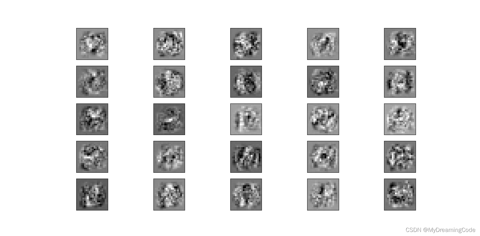
注意: 在运用神经网络的过程中,需要正则化,否则可能会引起过拟合现象。


 237
237


 被折叠的 条评论
为什么被折叠?
被折叠的 条评论
为什么被折叠?
 到【灌水乐园】发言


