pytorch深度学习（4）梯度下降算法

目录

         梯度下降算法

 代码1实现：

 画出关系图

随机梯度下降（Stochastic Gradient Descent）

代码2实现：（与上面类似）

---

上一次我们画出上面线性图所用的数据使用穷举法所求得的，但同时方法也存在弊端： 

       当权重w只有一个时，还能简单的用线性表示出来，

       如果出现两个权重时，如y_hat(w1,w2x)， 那就需要我们在一个平面上表示出来，所搜索的数量可能达到n^2个，

       如果权重出现两个以上时，10个权重就需要搜索n^10次。

所以我们换一种思路，采用分治法。

举个例子：当出现两个权重w时，首先我们将其划分为16个区域，如1所示，我们得出在红色框内取得最小值，紧接着，我们同样对红色框内的区域进行划分，如2所示16个区域，得出更准确的最小区域所代表的权重组合。

1

2

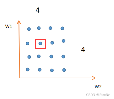
       这样一来，原本需要16*16=256次的搜索，现在变成只需要16+16=32次。

       但是，这种方法同样存在缺陷，因为我们的cost function（代价函数），并不完全像图3所示这样的凸函数，有可能是像图4这样的非凸函数，所以导致我们所找的最优值并不是全局最优，而是局部最优。

3

4

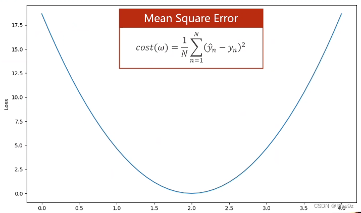
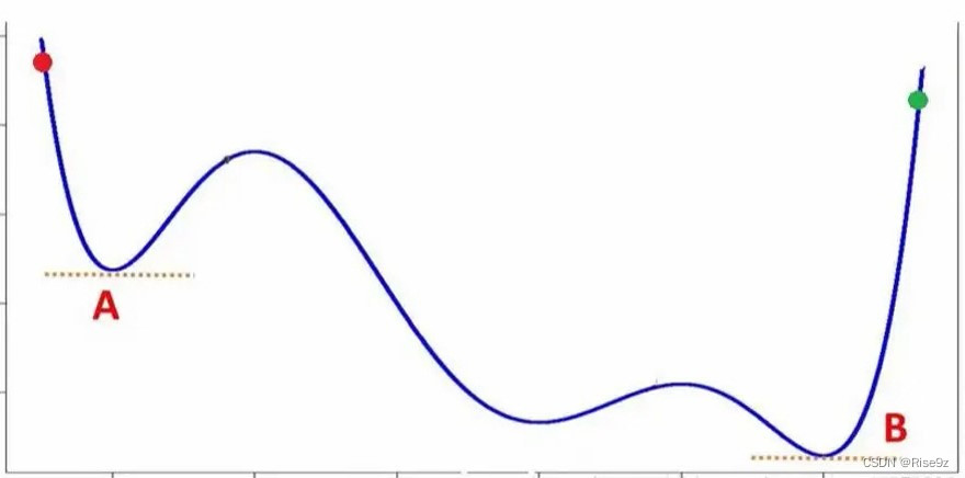
 因此，引出我们所要讨论的优化问题，去求得函数的最小值w*。

梯度下降算法

 

      初始点（Initial Guess）  到达全局的最小值（Global cost minimun）的最佳权重 w 

      移动方向：通过目标函数对权重求导，如果求得的导数>0，说明函数值再增加，函数往x正方向移动；如果导数<0，说明函数值在减小，函数往x负方向移动。

      对于上面梯度来说，我们需要到达最低点，就需要往x负方向移动，所以取负的导数。

 所以，在梯度下降算法里，我们用来更新权重的方法如上方所示（Update）    a是学习率

该方法就是前面我们讲的贪心法。

那我们前面也说过了，贪心法 求得的最优点是存在弊端的，它有可能只是局部最优的，而不是我们所要的全局最优。

---

但是，为什么梯度下降算法仍然要采用这种方式呢？

是因为，后来研究发现，深度神经网络中的损失函数中并没有很多的局部最优点，很少。

存在一种特殊情况：鞍点  g=0

---

  

 接下来就是一步一步地进行迭代。

我们拿上次的损失函数进行求导，具体过程如下：

 代码1实现：

x_data = [1.0, 2.0, 3.0]
y_data = [2.0, 4.0, 6.0]

w = 3.0   # 设定初始权重


def forward(x):        # 定义前馈模型
    return x * w


def cost(xs, ys):         # 算cost   MSE
    cost = 0
    for x, y in zip(xs, ys):          # for写个循环 zip拼装
        y_pred = forward(x)
        cost += (y_pred - y) ** 2            # 损失函数
    return cost / len(xs)               # 除以样本数量


def gradient(xs, ys):                  # 计算梯度
    grad = 0                         # 初始化
    for x, y in zip(xs, ys):
        grad += 2 * x * (x * w - y)            # 求和 累加过程
    return grad / len(xs)                        # 除以样本数量


print('Predict(before training)', 4, forward(4))
for epoch in range(100):
    cost_val = cost(x_data, y_data)                # 当前的损失值
    grad_val = gradient(x_data, y_data)                # 求梯度
    w -= 0.01 * grad_val                                   # 更新 Updata
    print('Epoch', epoch, 'w', w, 'loss', cost_val)        # 输出
print('Predict (after training)', 4, forward(4))

 最后的效果：

 我们可以看到 随着更新次数Epoch的增多 cost不断减小，趋近于0；

  同时权重w也稳定在2.00

最终我们得出，如果学习四个小时，得到的分数为8分

---

 画出关系图

也可以利用matplotlib画出epoch与cost的关系。

    epoch_list.append(epoch)
    cost_list.append(cost_val)
    plt.plot(epoch_list, cost_list)  # 绘制线性图
    plt.ylabel('cost')
    plt.xlabel('epoch')
    plt.show()

 出来的效果图如下（ cost 趋近于0）：

---

 完整代码：

import matplotlib.pyplot as plt

x_data = [1.0, 2.0, 3.0]
y_data = [2.0, 4.0, 6.0]

w = 1.0   # 设定初始权重
epoch_list = []  # 准备两个空列表
cost_list = []


def forward(x):        # 定义前馈模型
    return x * w


def cost(xs, ys):     # 算cost   MSE
    cost = 0
    for x, y in zip(xs, ys):     # for写个循环 zip拼装
        y_pred = forward(x)
        cost += (y_pred - y) ** 2    # 损失函数
    return cost / len(xs)       # 除以样本数量


def gradient(xs, ys):          # 计算梯度
    grad = 0                    # 初始
    for x, y in zip(xs, ys):
        grad += 2 * x * (x * w - y)    # 求和 累加过程
    return grad / len(xs)         # 除以样本数量


print('Predict(before training)', 4, forward(4))
for epoch in range(100):
    cost_val = cost(x_data, y_data)        # 当前的损失值
    grad_val = gradient(x_data, y_data)    # 求梯度
    w -= 0.01 * grad_val     # 更新 Updata
    print('Epoch', epoch, 'w', w, 'loss', cost_val)   # 输出
    epoch_list.append(epoch)
    cost_list.append(cost_val)
    plt.plot(epoch_list, cost_list)  # 绘制线性图
    plt.ylabel('cost')
    plt.xlabel('epoch')
    plt.show()
print('Predict (after training)', 4, forward(4))

---

平均加权均值

没有趋于0？   降低学习率

随机梯度下降（Stochastic Gradient Descent）

 随机梯度下降是指在总数的N里随机选一个，拿单个样本的损失函数，对权重求导，进行更新。

代码2实现：（与上面类似）

x_data = [1.0, 2.0, 3.0]
y_data = [2.0, 4.0, 6.0]

w = 1.0   # 设定初始权重


def forward(x):        # 定义前馈模型
    return x * w


def loss(x, y):     # 算loss   MSE
    y_pred = forward(x)
    return (y_pred - y) ** 2


def gradient(x, y):          # 计算梯度
    return 2 * x * (x * w - y)


print('Predict(before training)', 4, forward(4))
for epoch in range(100):
    for x, y in zip(x_data, y_data):        # 当前的损失值
        grad = gradient(x, y)    # 求梯度
        w -= 0.01 * grad     # 更新 Updata
        print("\tgrad:", x, y, grad)   # 输出
    print("progress:", epoch, "w=", w, "loss", 1)
print('Predict (after training)', 4, forward(4))

变换成单个样本进行训练

效果图如下：（最终结果与上面一致）

---

深度学习里

关于样本   ，（Batch）并行的话，性能低，时间低      代码1

              （Mini-Batch）批量的话，性能高，时间高     代码2

---