文献分享: 神经网络的热带几何分析

原论文
笔记(源文件)
笔记(PDF)
笔记(HTML)

$\text{1. }$热带几何$\text{\&}$热带代数

$\text{1.1. }$热带半环

1️⃣基本概念：集合$+$集合上的运算$\text{+}$单位元，即 ( K , ⊕ , ⊗ , 0 , 1 ) = ( R ∪ { − ∞ } , max ⁡ , + , − ∞ , 0 ) ({K,\oplus,\otimes,\mathbb{0},\mathbb{1}}){=}({\mathbb{R}{\cup}\{{-}{\infty} \},\max,{+},{-}{\infty},0}) (K,⊕,⊗,0,1)=(R∪{−∞},max,+,−∞,0)

1. 集合：所有实数加一个特殊元素(负无穷$-\infty$)，即 R ∪ { − ∞ } \mathbb{R}{\cup}\{{-}\infty\} R∪{−∞}
2. 运算：对 x , y ∈ R ∪ { − ∞ } x,y{\in}{\mathbb{R}{\cup}\{{-}\infty \}} x,y∈R∪{−∞}，热带加法 x ⊕ y = max ⁡ { x , y } x{\oplus}y{=}\max\{x,y\} x⊕y=max{x,y}，热带乘法$x\otimes y=x+y$
3. 单位元：$-\infty$是热带加的单位元 max ⁡ { x , − ∞ } = x \max\{x,{-}\infty\}{=}x max{x,−∞}=x，$0$是热带乘的单位元$x+0=x$

2️⃣基本性质：环❌$/$半环✅$/$半域✅

1. 为何是半环：满足以下运算定律

   运算律	对热带加法	对热带乘法
   交换律	max ⁡ { a , b } = max ⁡ { b , a } \max\{a,b\}{=}\max\{b,a\} max{a,b}=max{b,a}	$a+b=b+a$
   结合律	max ⁡ { max ⁡ { a , b } , c } = max ⁡ { a , max ⁡ { b , c } } \max\{\max\{a,b\},c\}{=}\max\{a,\max\{b,c\}\} max{max{a,b},c}=max{a,max{b,c}}	$a+(b+c)=(b+a)+c$

   • 分配律： a + max ⁡ { b , c } = max ⁡ { a + b , a + c } a{+}\max\{b,c\}{=}\max\{a{+}b,a{+}c\} a+max{b,c}=max{a+b,a+c}
2. 关于逆元：对热带半环，加法逆元❌$/$乘法逆元✅

   逆元类型	定义	对热带半环
   加法逆元	若$x\oplus y=0$则$y$为$x$加法逆元，记$y=-x$	不存在 max ⁡ { x , y } = − ∞ \max\{x,y\}{=}{-}{\infty} max{x,y}=−∞故不为环
   乘法逆元	若$x\otimes y=1$则$y$为$x$乘法逆元，记$y=x^{-1}$	存在$x+(-x)=0$故为半域，故可进行除法

   • 所谓环：在半环的基础上，所有元素都必须有其对应的加法逆元
   • 所谓半域：在半环的基础上，除了加法单位元以外的所有元素，都必须有其对应的乘法逆元

3️⃣热带函数：有理函数(热带多项式的热带商)$\leftarrow$多项式$\leftarrow$扩展运算

1. 运算扩展：热带幂和热带商

   运算	半环中	热带半环中	特殊的
   热带幂	$x^{\otimes a}=x\otimes \cdots \otimes x$	$x^{\otimes a}=ax$	$(-\infty {)}^{\otimes a}=-\infty$及$(-\infty {)}^{\otimes 0}=0$
   热带商	$a\oslash b=a\otimes b^{\otimes (-1)}$	$a\oslash b=a-b$	$\text{N/A}$

2. 热带多项式$\&$有理函数：令$\mathbf{x}=⟨x_1,...,x_d⟩$
   • 热带多项式：相当于多个线性函数(更精确地说，仿射函数)取最大值

     算式	结构	转换回常规运算	性质
     热带单项式	$L_i(\mathbf{x})=c_i\otimes x_1^{\otimes a_1}\otimes \cdots \otimes x_d^{\otimes a_d}$	$c_i+a_{i1}{x}_1+\cdots +a_{id}{x}_d$	线性函数
     热带多项式	$f(\mathbf{x})=L_1\oplus L_2\oplus \cdots \oplus L_r$	max ⁡ { L 1 ( x ) , . . . , L r ( x ) } \max\{L_1(\mathbf{x}),...,L_r(\mathbf{x})\} max{L1​(x),...,Lr​(x)}	凸函数

   • 热带有理函数：热带多项式的热带商，且定义$f(\mathbf{x})\oslash g(\mathbf{x})=f(\mathbf{x})-g(\mathbf{x})$

     符号	定义	转换回常规运算	性质
     $h(\mathbf{x})$	$f(\mathbf{x})\oslash g(\mathbf{x})$	max ⁡ { L 1 , . . . , L r } − max ⁡ { L 1 ′ , . . . , L s ′ } \max\{L_1,...,L_r\}{-}\max\{L_1',...,L_s'\} max{L1​,...,Lr​}−max{L1′​,...,Ls′​}	两凸函数差($\text{DC}$函数)

   • 补充：对$\mathbf{x}=⟨x_1,...,x_d⟩$及${\mathbf{\alpha }}_{\mathbf{i}}=⟨a_{i1},...,a_{id}⟩$，多项式$c_i\otimes x_1^{\otimes a_{i1}}\otimes \cdots \otimes x_d^{\otimes a_{id}}$可简写为$c_i{\mathbf{x}}^{{\mathbf{\alpha }}_{\mathbf{i}}}$
3. 一些推广：函数集代数结构与向量值函数
   • 函数集的代数结构：注意，热带多项式可看作热带有理函数分母为$1=0$时

     集合	半环结构	半域
     $x_1,...,x_d$构成的所有热带多项式集	$(\mathbb{T}[x_1,...,x_d],\max ,+,-\infty ,0)$	❌
     $x_1,...,x_d$构成的所有热带有理函数集	$(\mathbb{T}(x_1,...,x_d),\max ,+,-\infty ,0)$	✅

   • 向量值函数：将不同的函数$/$多项式一次拼接

     向量函数类型	函数${\mathbb{R}}^{\mathbf{d}}\to {\mathbb{R}}^{\mathbf{p}}$的定义	补充
     热带多项式	$F_f:F(\mathbf{x})=(f_1(\mathbf{x}),...,f_p(\mathbf{x}))$	$\text{Pol}(d,p)$为所有$F_f:{\mathbb{R}}^d\to {\mathbb{R}}^p$函数集
     热带有理函数	$F_h:F(\mathbf{x})=(h_1(\mathbf{x}),...,h_p(\mathbf{x}))$	$\text{Rat}(d,p)$为所有$F_h:{\mathbb{R}}^d\to {\mathbb{R}}^p$函数集

$\text{1.2. }$热带超曲面与牛顿对偶

1️⃣热带超曲面

1. 定义：考虑热带多项式 f ( x ) = max ⁡ { L 1 ( x ) , . . . , L r ( x ) } f(\mathbf{x}){=}\max\{L_1(\mathbf{x}),...,L_r(\mathbf{x})\} f(x)=max{L1​(x),...,Lr​(x)}
   
   • 形式定义： T ( f ) = { x ∈ R d ∣ c i x α i = c j x α j = f ( x ) , i ≠ j } \mathcal{T}(f){=}\{\mathbf{x}{\in}\mathbb{R}^d\mid{}c_i\mathbf{x}^{\boldsymbol{\alpha_i}}{=}c_j\mathbf{x}^{\boldsymbol{\alpha_j}}{=}f(\mathbf{x}),i{\neq}j\} T(f)={x∈Rd∣ci​xαi​=cj​xαj​=f(x),i=j}，当$d=2$时从热带超曲面退化为热带曲线
   • 直观理解：多项式由最高平面 max ⁡ { L 1 ( x ) , . . . , L r ( x ) } \max\{L_1(\mathbf{x}),...,L_r(\mathbf{x})\} max{L1​(x),...,Lr​(x)}拼接成，热带超曲面即两最高平面连接处
   • 基本含义：在某点$\mathbf{x}$至少两单项式同时取得最大值，即 L i ( x ) = L j ( x ) = max ⁡ { L 1 ( x ) , . . . , L r ( x ) } L_i(\mathbf{x}){=}L_j(\mathbf{x}){=}\max\{L_1(\mathbf{x}),...,L_r(\mathbf{x})\} Li​(x)=Lj​(x)=max{L1​(x),...,Lr​(x)}
2. 本质：将 f ( x ) = max ⁡ { L 1 ( x ) , . . . , L r ( x ) } f(\mathbf{x}){=}\max\{L_1(\mathbf{x}),...,L_r(\mathbf{x})\} f(x)=max{L1​(x),...,Lr​(x)}划分为多个凸胞腔
   • 直观理解：每个凸胞腔都是一个单项式“称霸”的区域，即每个凸胞腔内$f(\mathbf{x})$可用一单项式精确描述
   • 形式定义：单项式$c_j{\mathbf{x}}^{{\alpha }_j}$取得最大值的胞腔是 { x ∈ R d ∣ c j + α j T x ≥ c i + α i T x , ∀ i ≠ j } \{\mathbf{x}{\in}\mathbb{R}^d\mid{}c_j{+}{\boldsymbol{\alpha_j}}^{T}\mathbf{x}{\geq}c_i{+}{\boldsymbol{\alpha_i}}^{T}\mathbf{x},\forall{i{\neq}j}\} {x∈Rd∣cj​+αj​Tx≥ci​+αi​Tx,∀i=j}

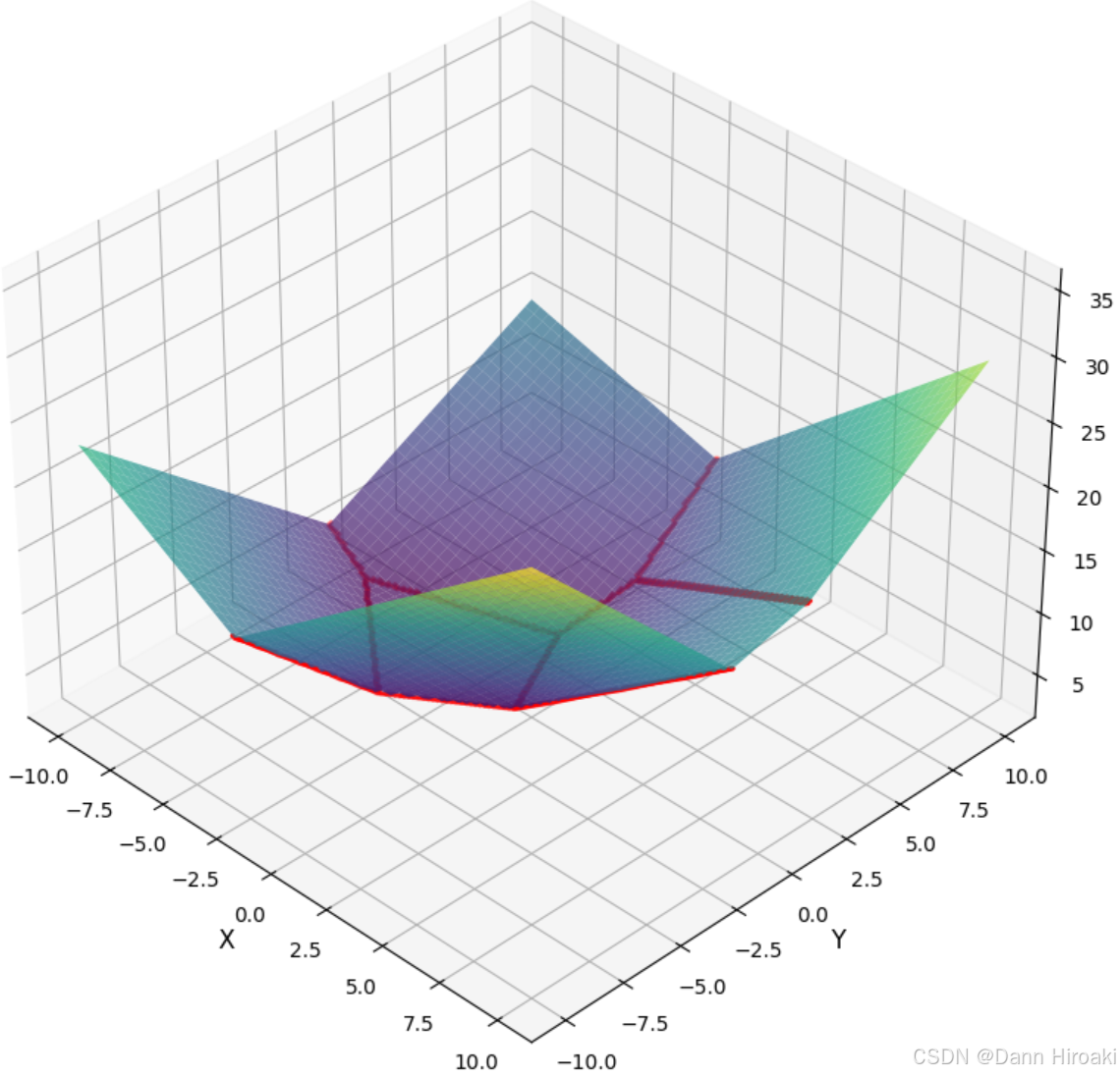
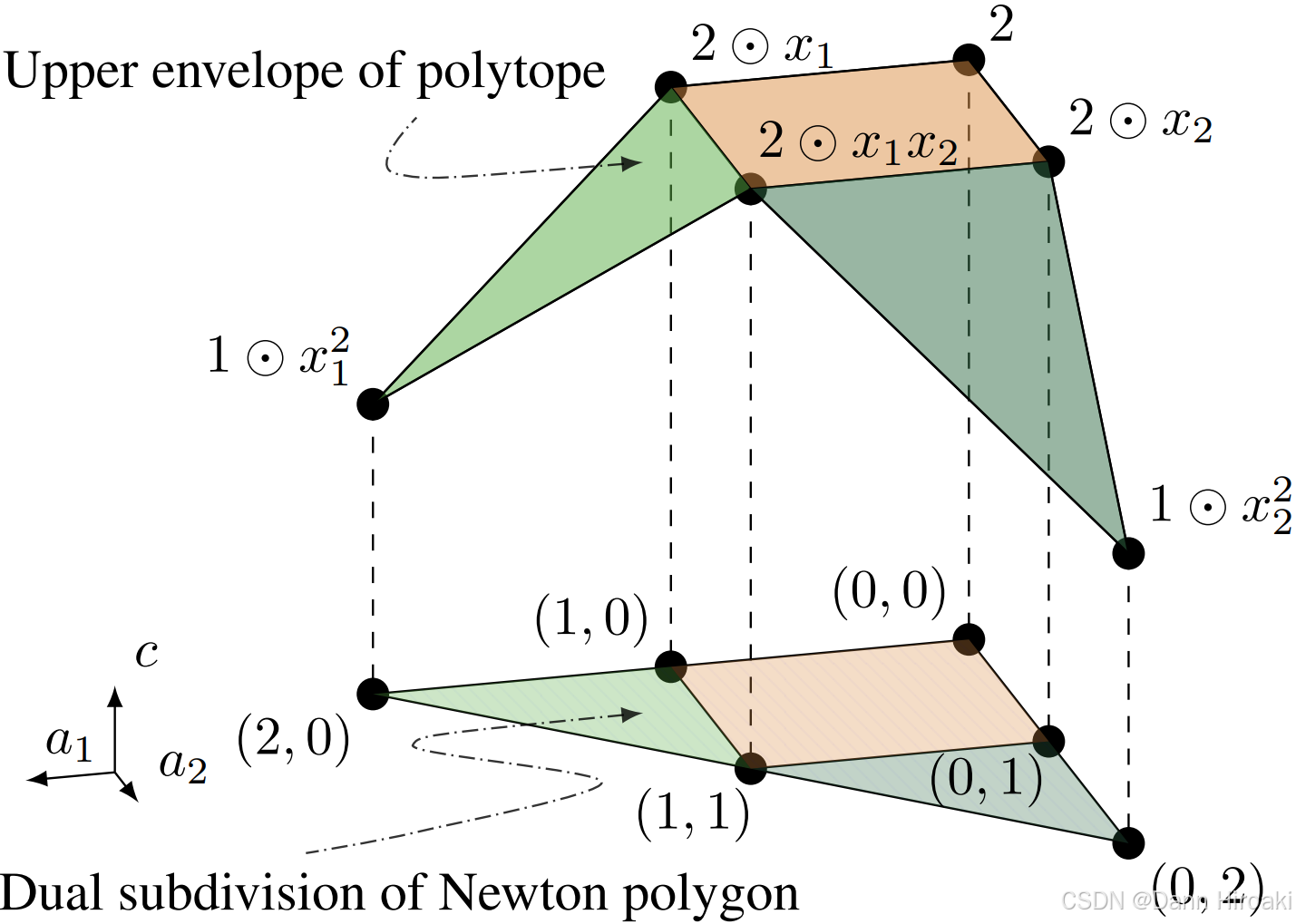
2️⃣牛顿多边形及牛顿对偶

1. 第一步：以$f(x_1,x_2)=(1\otimes x_1^2)\oplus (1\otimes x_2^2)\oplus (2\otimes x_1\otimes x_2)\oplus (2\otimes x_1)\oplus (2\otimes x_2)\oplus (2)$为例，提取因子

   单项式	${\mathbf{x}}_1$次方	${\mathbf{x}}_2$次方	常数项	指数点$\mathbf{\alpha }$	$\mathbf{c}$
   $1\otimes x_1^2$	$2$	$0$	$1$	${\alpha }_1=(2,0)$	$c_1=1$
   $1\otimes x_2^2$	$0$	$2$	$1$	${\alpha }_2=(0,2)$	$c_2=1$
   $2\otimes x_1\otimes x_2$	$1$	$1$	$2$	${\alpha }_3=(1,1)$	$c_3=2$
   $2\otimes x_1$	$1$	$0$	$2$	${\alpha }_4=(1,0)$	$c_4=2$
   $2\otimes x_2$	$0$	$1$	$2$	${\alpha }_5=(0,1)$	$c_5=2$
   $2$	$0$	$0$	$2$	${\alpha }_6=(0,0)$	$c_6=2$

2. 之后步：(注意所谓上表面，即表面法向量与$d$维中从最后一维$/$高度维夹角为锐角)
   

   操作	描述
   牛顿多边形$\Delta (f)$	取所有指数点$\alpha$的凸包(相当于用橡皮筋围住最外围点)
   多面体$\mathcal{P}(f)$	基于牛顿多边形，在$\alpha$基础上增加一个值为$c$的维度，成为$({\mathbf{\alpha }}_{\mathbf{i}},c_i)$
   对偶细分$\delta (f)$	将多面体$\mathcal{P}(f)$上表面的边和顶点，垂直投影回到底部牛顿多边形$\Delta (f)$

3. 最后步：对牛顿多边形$\Delta (f)$上的对偶细分$\delta (f)$，建立对偶细分$\delta (f)$和热带超曲面$\mathcal{T}(f)$的联系

   偶细分$\mathbf{\delta }(\mathbf{f})$	对应超曲面$\mathcal{T}(\mathbf{f})$	含义	$\mathbf{\delta }(\mathbf{f})$示例	对应$\mathcal{T}(\mathbf{f})$示例
   $k$维面	$(d-k)$维面	$k+1$个$L_i$打平	$\text{N/A}$	$\text{N/A}$
   边$(k=1)$	折痕$(k=1/d=2)$	两$L_i$打平	线$(1,0)\to (0,0)$	折痕($2\otimes x_1=2$)
   顶点$(k=0)$	线性区$(k=0/d=2)$	一$L_i$主导	点$(1,0)$	线性区($2\otimes x_1$主导)

   • 对偶定理：$\mathcal{T}(f)$线性区域数$=\mathcal{P}(f)$上表面顶点数$\le \mathcal{P}(f)$总顶点数

3️⃣线性区域：

1. 含义：$F$定义域中保持其线性的最大的连通子集，即同一线性区域内不同的两点都线性可达
2. 性质：当$F$为热带多项式(凸函数)时其线性区域为凸，当$F$为热带有理函数($\text{DC}$函数)时其线性区域非凸
3. 意义：$F$线性区域数量记为$\mathcal{N}(F)$，一个神经网络能划分出更多线性区域，去拟合能力更强

$\text{1.3. }$热带多项式的几何学描述

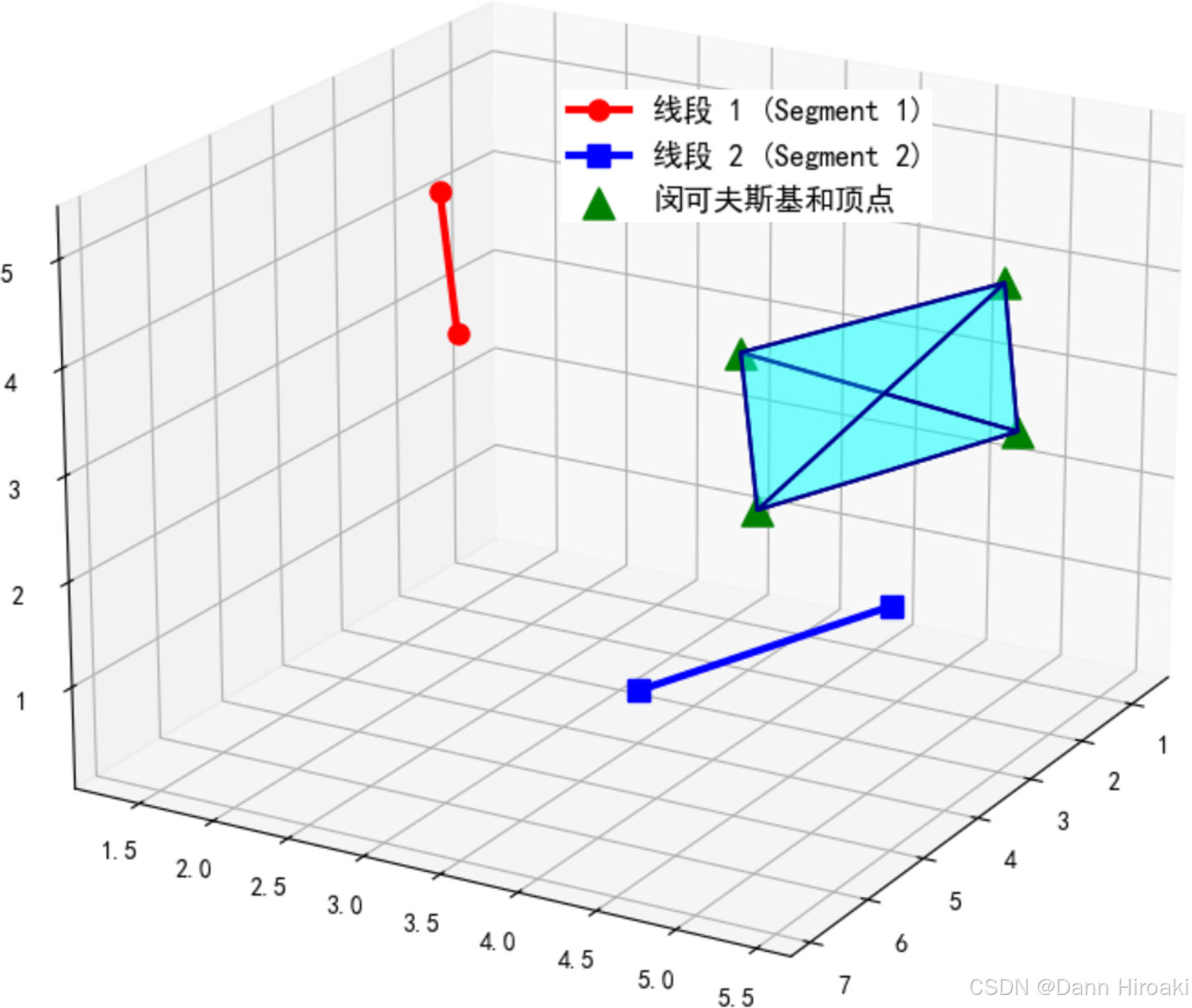
0️⃣闵可夫斯基和：形式定义与一些延申

1. 形式定义：对两集合$P_1/P_2$而言，其$\text{Minkowski}$和为 P 1 + P 2 := { x 1 + x 2 ∣ x 1 ∈ P 1 , x 2 ∈ P 2 } P_1{+}P_2 \mathrel{\text{:=}}\{x_1{+}x_2 \mid x_1{\in}P_1,x_2{\in}P_2\} P1​+P2​:={x1​+x2​∣x1​∈P1​,x2​∈P2​}
2. 直观理解：将形状$P_2$的原点，在形状$P_1$每个点上移动，移动过程中$P_2$扫描的区域即$\text{Minkowski}$和
3. 对多面体：多面体$\mathcal{P}(f)$合$\mathcal{P}(g)$的$\text{Minko.}$和，即顶点集$\mathcal{V}(\mathcal{P}(f))$和$\mathcal{V}(\mathcal{P}(g))$的$\text{Minko.}$和，再求凸包
4. 一些扩展：两个(或多个)线段的$\text{Minkowski}$和(一线段每个点与另一线段每个点相加)，为带状多面体
   

1️⃣构建与变换：热带多项式的几何学

1. 单项式与顶点：
   • 结构上：$f$一单项式$L_i=c_i+a_{i1}{x}_1+\cdots +a_{id}{x}_d\stackrel{对应}{\iff }\mathcal{P}(f)$一生成顶点$({\mathbf{\alpha }}_{\mathbf{i}},c_i)=(a_{i1},...,a_{id},c_i)$
   • 运算上：$f$单项式的热带运算$\stackrel{等价}{\iff }$对$\mathcal{P}(f)$顶点的几何变换，具体如下

     单项式的热带运算	转为常规运算	相当于对多面体中…
     $L_1\otimes \cdots \otimes L_n$	$L_1+\cdots +L_n$	将$({\mathbf{\alpha }}_{\mathbf{i}},c_i)$求和变成求$({\mathbf{\alpha }}_1+\cdots +{\mathbf{\alpha }}_{\mathbf{n}},c_1+\cdots +c_n)$
     $L_i^{\otimes a}$	$a{L}_i$	放缩$({\mathbf{\alpha }}_{\mathbf{i}},c_i)$成$(a{\mathbf{\alpha }}_{\mathbf{i}},a{c}_i)$

2. 单项式到多项式
   • 结构上：多个单项式热带相加$\stackrel{等价}{\iff }$多个顶点求凸包以生成成多面体
   • 运算上：$f=L_1\oplus \cdots \oplus L_n$可转化为 f = max ⁡ { L 1 , . . . , L n } f{=}\max\{L_1,...,L_n\} f=max{L1​,...,Ln​}，即求$\{({\mathbf{\alpha }}_1,c_1),...,({\mathbf{\alpha }}_{\mathbf{n}},c_n)\}$凸包
3. 多项式与多面体：
   • 热带幂$f^{\otimes a}$：相当于缩放，即$\mathcal{P}(f^{\otimes a})=a\mathcal{P}(f)$

     领域	操作	解释
     热带运算	热带幂$f^{\otimes a}$	相当于$a\times f$，即每个单项式系数$c_i$和指数 α i = { a i 1 , . . , a i d } \boldsymbol{\alpha_i}{=}\{a_{i1},..,a_{id}\} αi​={ai1​,..,aid​}乘上$a$
     几何变换	缩放	每个顶点$({\mathbf{\alpha }}_{\mathbf{i}},c_i)$变为$(a{\mathbf{\alpha }}_{\mathbf{i}},a{c}_i)$，即每个顶点都相对原点拉伸$a$倍

   • 热带积$f\otimes g$：相当于闵可夫斯基和，即$\mathcal{P}(f\otimes g)=\mathcal{P}(f)+\mathcal{P}(g)$

     领域	操作	解释
     热带运算	热带积$f\otimes g$	$f$每个单项式与$g$每个单项式热带乘(相加)再热带加(求$\max$)
     几何变换	多面体$\text{Minko.}$和	$\mathcal{P}(f)$每个顶点与$\mathcal{P}(g)$每个顶点坐标依次相加，再求凸包

   • 热带和$f\oplus g$：相当于顶点联合的凸包，即$\mathcal{P}(f\oplus g)=\text{Conv}(\mathcal{V}(\mathcal{P}(f))\cup \mathcal{V}(\mathcal{P}(g)))$

     领域	操作	解释
     热带运算	热带积$f\oplus g$	$f$和$g$各自的多项式合在一起，再求合一起后的最大值
     几何变换	顶点联合的凸包	$\mathcal{P}(f)$与$\mathcal{P}(g)$中所有顶点合在一起，对合一起后的点集求凸包

2️⃣理论保证：如何界定新生成多面体的顶点数

1. $\text{Gritzmann-Sturmfels}$定理：生成多面体最多多少个顶点
   • 参数说明：$d+1$表示多面体$P_1,...,P_k$所处空间的维度，$m$为收集所有$P_i$棱后非平行棱的总数
   • 定理内容：令多面体$P_1,...,P_k$进行$\text{Minkowski}$和后新多面体顶点数为$N$，则$N\le 2\sum _{j=0}^d{\mathbf{C}}_{m-1}^j$
   • 取等条件：每个多面体$P_i$都为带状多面体，且构成每个$P_i$的线段都处于一般位置
2. 定理的关键推论：新生成多面体上表面有多少顶点，即多项式有多少线性区域数
   • 条件改变：$P_1,...,P_k$从任意形状的多面体限定为了带状多面体，
   • 结论改变：$P_1,...,P_k$进行$\text{Minkowski}$和后新多面体上表面顶点数为$N^{\prime }$，则$N^{\prime }\le \sum _{j=0}^d{\mathbf{C}}_m^j$
   • 取等条件：$P_i$所有$m$条线段都处于一般位置，新多面体($d+1$维)顶点投影回$d$维后都处于一般位置
3. (补充)关于一般位置：即任意$k$个点不会被维度$\le k-2$的空间容纳，例如四点不共面，三点不共线

$\text{2. }$神经网络的热带几何$\text{\&}$代数

$\text{2.1. }$神经网络及其假设

1️⃣神经网络的数学模型：定义一个共$L^{(n)}$层全连接的前馈网络 %以下内容我对原文的符号体系做了一些改变，力求符合我自己的符号体系，在审查时请忽略符号体系的改变

1. 对于每一层$L^{(i)}$：
   • 结构：输入$d_{i-1}$维的${\text{x}}^{(i-1)}$后输出$d_i$维的${\text{x}}^{(i)}$，每层可学习参数有权重矩阵${\mathbf{A}}_{d_i\times d_{i-1}}$及偏置向量${\mathbf{b}}_{d_i}$
   • 运算：先将${\text{x}}^{(i-1)}$输入仿射变换${\rho }_i\left({\text{x}}^{(i-1)}\right)={\mathbf{A}}_{d_i\times d_{i-1}}{\text{x}}^{(i-1)}+{\mathbf{b}}_{d_i}$再激活${\text{x}}_i={\sigma }_i\left({\rho }_i\left({\text{x}}^{(i-1)}\right)\right)$
   • 补充：本文${\sigma }_i$采用广义$\text{ReLU}$(详见下)，因为其为最典型的激活函数，也方便用热带代数描述
2. 对于所有$L^{(n)}$层：
   • 结构：$\nu =({\sigma }_n\circ {\rho }_n)\circ ({\sigma }_{n-1}\circ {\rho }_{n-1})\circ \cdots \circ ({\sigma }_1\circ {\rho }_1)$即$\nu \left({\text{x}}^{(0)}\right)={\text{x}}^{(n)}$，但不会$\text{Softmax}\left({\text{x}}^{(n)}\right)$一下
   • 运算：${\text{x}}^{(0)}\stackrel{{\sigma }_1\left({\rho }_1\left({\text{x}}^{(0)}\right)\right)}{\to }{\text{x}}^{(1)}\stackrel{{\sigma }_2\left({\rho }_2\left({\text{x}}^{(1)}\right)\right)}{\to }{\text{x}}^{(2)}\to \cdots \to {\text{x}}^{(n-1)}\stackrel{{\sigma }_n\left({\rho }_n\left({\text{x}}^{(n-1)}\right)\right)}{\to }{\text{x}}^{(n)}$

2️⃣三条较温和的假设：使神经网络行为能严格对应热带运算

1. 对权重矩阵：${\mathbf{A}}_{d_i\times d_{i-1}}$每个权重都是整数，这种假设是温和的(见下例)，对应了热带单项式的指数
   $\left[\begin{array}{cc}0.5& 1.2\\ 2.5& \sqrt{2}\end{array}\right](实数)\stackrel{用有理数估计无理数}{\to }\left[\begin{array}{cc}0.5& 1.2\\ 2.5& 1.4\end{array}\right](有理数)\stackrel{通分以去除小数点}{\to }\left[\begin{array}{cc}5& 12\\ 25& 14\end{array}\right](整数)$
2. 对偏置向量：${\mathbf{b}}_{d_i}$的每个值都是实数，对应热带单项式的系数$c$
3. 广义$\text{ReLU}$：即 σ ( x j ) = max ⁡ { x j , t j } = x j ⊕ t j \sigma{(x_j)}{=}\max\{x_j,t_j\}{=}x_j{\oplus}t_j σ(xj​)=max{xj​,tj​}=xj​⊕tj​(逐个应用在$\mathbf{x}$每维)，非线性激活可用热带运算表述
   • 可退化为其它的激活函数：当$t=0$时退化为普通$\text{ReLU}$函数，当$t=-\infty$时$\sigma (x)=x$
   • 不可退化为平滑激活函数：如$\text{sigmoid/tanh}$等

$\text{2.2. }$神经网络的热带代数

1️⃣从神经网络到热带有理函数：写在前面

1. 灵感所在：热带多项式为凸$\stackrel{两凸之差非凸}{\to }$热带有理函数非凸；神经网络也非凸，是否等于热带有理函数
2. 计算要素：$\mathbf{A}\text{x}+\mathbf{b}$过程中，神经网络中的参数最终会到热带多项式的哪里

   $\mathbf{A}\text{x}+\mathbf{b}$过程	热带代数中	备注
   $\mathbf{A}\text{x}$中的$a_{kj}{x}_j$	$(x_j{)}^{\otimes a_{kj}}$	权重参数$\stackrel{变为}{\to }$热带多项式中的幂，幂必为整数故权重只能为整数
   $+\mathbf{b}$中的$+b_k$	$\otimes b_k$	偏置参数$\stackrel{变为}{\to }$热带多项式的系数

2️⃣从神经网络到热带有理函数：递归证明(全文最核心部分)

1. 基础步骤：原始输入${\mathbf{x}}^{(0)}$，经过第$1$层$L^{(1)}$的输出${\mathbf{x}}^{(1)}$是怎么样的
   • 每层输出：得到${\mathbf{x}}^{(1)}=\max \left\{\left({\mathbf{A}}_{d_1\times d_0}{\text{x}}^{(0)}+{\mathbf{b}}_{d_1}\right),{\mathbf{t}}_{d_1}\right\}$
   • 权重分解：提取${\mathbf{A}}_{d_1\times d_0}$绝对值以分解为${\mathbf{A}}_{d_1\times d_0}^{(+)}$和${\mathbf{A}}_{d_1\times d_0}^{(-)}$，且${\mathbf{A}}_{d_1\times d_0}={\mathbf{A}}_{d_1\times d_0}^{(+)}-{\mathbf{A}}_{d_1\times d_0}^{(-)}$
   • 恒等变换：得到${\mathbf{x}}^{(1)}=\max \left\{\left({\mathbf{A}}_{d_1\times d_0}^{(+)}{\text{x}}^{(0)}+{\mathbf{b}}_{d_1}\right),\left({\mathbf{A}}_{d_1\times d_0}^{(-)}{\text{x}}^{(0)}+{\mathbf{t}}_{d_1}\right)\right\}-{\mathbf{A}}_{d_1\times d_0}^{(-)}{\text{x}}^{(0)}$
   • 热带表示：设置${\mathbf{x}}^{(1)}=F^{(1)}\left({\text{x}}^{(0)}\right)-G^{(1)}\left({\text{x}}^{(0)}\right)$，(如下表)${\mathbf{x}}^{(1)}$每一维都是热带有理函数

     项(共${\mathbf{d}}_{\mathbf{i}}$维)	热带算式	热带多项式
     $F^{(1)}$第$k$维	$\left[b_k\otimes \left(\underset{j}{⨂}{\left(x_j^{(0)}\right)}^{\otimes a_{kj}^{(+)}}\right)\right]\oplus \left[t_k\otimes \left(\underset{j}{⨂}{\left(x_j^{(0)}\right)}^{\otimes a_{kj}^{(-)}}\right)\right]$	✅
     $G^{(1)}$第$k$维	$\left(\underset{j}{⨂}{\left(x_j^{(0)}\right)}^{\otimes a_{kj}^{(-)}}\right)$	✅

   • 最终结论：输出${\mathbf{x}}^{(1)}$每一维严格满足热带有理函数定义，即${\mathbf{x}}^{(1)}$每一维都是热带有理函数
2. 归纳步骤：第$i$层$L^{(i)}$的输出${\mathbf{x}}^{(i)}$，经过第$i+1$层$L^{(i+1)}$的输出${\mathbf{x}}^{(i+1)}$是怎么样的

   符号	值	每维依然是热带多项式
   $H^{(i+1)}$	$\left({\mathbf{A}}_{d_{i+1}\times d_i}^{(+)}{F}^{(i)}+{\mathbf{A}}_{d_{i+1}\times d_i}^{(-)}{G}^{(i)}+{\mathbf{b}}_{d_{i+1}}\right)$	✅
   $G^{(i+1)}$	$\left({\mathbf{A}}_{d_{i+1}\times d_i}^{(-)}{F}^{(i)}+{\mathbf{A}}_{d_{i+1}\times d_i}^{(+)}{G}^{(i)}\right)$	✅
   $F^{(i+1)}$	$\max \left\{H^{(i+1)},\left(G^{(i+1)}+{\mathbf{t}}_{d_{i+1}}\right)\right\}$	✅

   • 仿射：${\rho }^{(i+1)}={\mathbf{A}}_{d_{i+1}\times d_i}{\mathbf{x}}^{(i)}+{\mathbf{b}}_{d_{i+1}}=H^{(i+1)}-G^{(i+1)}$
   • 激活：${\mathbf{x}}^{(i+1)}=\max \left\{H^{(i+1)},\left(G^{(i+1)}+{\mathbf{t}}_{d_{i+1}}\right)\right\}-G^{(i+1)}=F^{(i+1)}-G^{(i+1)}$，为一个热带有理函数
   • 结论：每一层的输出${\mathbf{x}}^{(i)}$的每一维都是一个热带有理函数
3. 最终结论：函数$\nu$满足三条假设的神经网络$\stackrel{等价于}{\iff }\nu$可以被看作一个热带有理函数

3️⃣从神经网络到热带有理函数：结论扩展

1. 引入上界：视热带函数$f\oslash g$为$n$层神经网络，则 n ≤ max ⁡ { ⌈ log ⁡ 2 r f ⌉ , ⌈ log ⁡ 2 r g ⌉ } + 2 n{\leq}\max\left\{\lceil\log_{2}{r_f}\rceil,\lceil\log_{2}{r_g}\rceil\right\}{+}2 n≤max{⌈log2​rf​⌉,⌈log2​rg​⌉}+2($r$为单项式数量)
2. 新的等价：现引入并考虑连续分段线性函数，则以下三者任意二者互相等价
   • 整数系数连续分段线性函数$f-g$
   • 热带有理函数$f\oslash g$
   • 满足三条假设的神经网络
3. 更强等价：去除权重为整数的限制的神经网络$\stackrel{可视作}{\Rightarrow }$热带有理符号映射
   • 热带符号函数：即$\phi \left(x\right)=\underset{k=1}{\overset{m}{⨁}}\left(b_k\otimes \left(\underset{j=1}{\overset{n}{⨂}}{x}_j^{a_{kj}}\right)\right)$，$a_{kj}$为实数(多项式中只能是整数)
   • 热带有理符号映射：类似于热带有理函数，被定义为连哥哥热带符号函数的热带商${\phi }_1\oslash {\phi }_2$
   • 一些讨论：本文非要使用热带符号函数的“退化”热带多项式，因为只有后者才属于热带几何范畴

$\text{2.3. }$神经网络的热带几何

$\text{2.3.1. }$决策边界的热带几何性质

1️⃣决策边界的概念

1. 评分函数：变换神经网络输出${\text{x}}^{(n)}$以得到评分$s\left({\text{x}}^{(n)}\right)$，如$\text{Softmax}\left({\text{x}}^{(n)}\right)/\text{Sigmiod}\left({\text{x}}^{(n)}\right)$
2. 决策规则：用于分类，比如二元分类中$s\left({\text{x}}^{(n)}\right)$大于阈值$c$就归为一类，小于阈值$c$就归为另一类
3. 决策边界：使评分等于决策阈值的神经网络输入集$\mathcal{B}:=\left\{{\text{x}}^{(0)}\in {\mathbb{R}}^{d_0}|s\left(\nu \left({\text{x}}^{(0)}\right)\right)=s\left({\text{x}}^{(n)}\right)=c\right\}$

2️⃣决策边界的热带几何性

0. 前提条件：所有研究是神经网络$\nu$是怎么样的
   • $\nu$满足前面所提到的三个假设，即权重为整数$/$偏置量为实数$/$激活函数为广义$\text{ReLU}$
   • $\nu$最后一层$L^{(n)}$只进行仿射变换不激活，即令${\mathbf{t}}_{d_n}=-\infty$使$\sigma \left({\text{x}}^{(n)}\right)=\max \left\{{\text{x}}^{(n)},-\infty \right\}={\text{x}}^{(n)}$
   • $\nu$可写为两热带多项式$f\left({\text{x}}^{(0)}\right)$和$g\left({\text{x}}^{(0)}\right)$的热带商，即$\nu \left({\text{x}}^{(0)}\right)=f\left({\text{x}}^{(0)}\right)\oslash g\left({\text{x}}^{(0)}\right)$
1. 结论一：决策边界划分出来的正区域的数量，存在一个天然的上界$\mathcal{N}(f)$
   • 正区：即评分大于阈值$s\left(\nu \left({\text{x}}^{(0)}\right)\right)\ge c$，即$f\left({\text{x}}^{(0)}\right)\ge g\left({\text{x}}^{(0)}\right)+s^{-1}(c)$的区域，含义如下

     结构	如何理解
     $f\left({\text{x}}^{(0)}\right)$	好比一个"地表"(多项式)，由$\mathcal{N}(f)$个平坦"斜面"(某个单项式)拼接而成
     $g\left({\text{x}}^{(0)}\right)+s^{-1}(c)$	好比一个"水面"(多项式)，由$\mathcal{N}(g)$个平坦"斜面"(某个单项式)拼接而成
     正区	“地表"没有被"水面"淹没的地方，即好比"孤岛”

   • 结论：对$f\left({\text{x}}^{(0)}\right)$每块"斜面"，或被淹没$/$与其他"斜面"一起构成"孤岛"，故"孤岛"定少于"斜面"
2. 结论二：神经网络的决策边界$\mathcal{B}$，被一个更完整的热带超曲面包含
   • 上表面：即$h\left({\text{x}}^{(0)}\right)=\max \left\{f\left({\text{x}}^{(0)}\right),\left(g\left({\text{x}}^{(0)}\right)+s^{-1}(c)\right)\right\}$，好比“可见地貌”(“水面”$+$“孤岛”)
   • 超曲面：即$\mathcal{T}\left(h\left({\text{x}}^{(0)}\right)\right)$，表示“可见地貌”上的所有"斜面"的"棱线"，这些"棱线"分为三类

     类型	如何理解
     “海岸线”	即决策边界$\mathcal{B}$，也就是$f\left({\text{x}}^{(0)}\right)=g\left({\text{x}}^{(0)}\right)+s^{-1}(c)$"地表"和"水面"等高的地方
     “陆地线”	$\mathcal{T}\left(f\left({\text{x}}^{(0)}\right)\right)$的被“海岸线”(决策边界)截去的上半部分
     “海洋线”	$\mathcal{T}\left(g\left({\text{x}}^{(0)}\right)+s^{-1}(c)\right)$的被“海岸线”(决策边界)截去的下半部分

   • 结论：神经网络的决策边界$\mathcal{B}$被热带超曲面$\mathcal{T}(h)$容纳，即$\mathcal{B}\subseteq \mathcal{T}(h)$

$\text{2.3.2. }$神经网络的热带几何演化

1️⃣知识回顾：递推公式与几何变换

1. 逐层递推：设神经网络$L^{(i)}$层输出为两热带多项式的热带商${\mathbf{x}}^{(i)}=F^{(i)}\left({\text{x}}^{(i-1)}\right)-G^{(i)}\left({\text{x}}^{(i-1)}\right)$，则
   $\{\begin{array}{l}{G}^{(i+1)}=\left({\mathbf{A}}_{d_{i+1}\times d_i}^{(-)}{F}^{(i)}+{\mathbf{A}}_{d_{i+1}\times d_i}^{(+)}{G}^{(i)}\right)\\ \\ F^{(i+1)}=\max \left\{\left({\mathbf{A}}_{d_{i+1}\times d_i}^{(+)}{F}^{(i)}+{\mathbf{A}}_{d_{i+1}\times d_i}^{(-)}{G}^{(i)}+{\mathbf{b}}_{d_{i+1}}\right),\left({\mathbf{A}}_{d_{i+1}\times d_i}^{(-)}{F}^{(i)}+{\mathbf{A}}_{d_{i+1}\times d_i}^{(+)}{G}^{(i)}+{\mathbf{t}}_{d_{i+1}}\right)\right\}\end{array}$
2. 几何变换：多项式$f$的运算$\stackrel{等价地体现}{\iff }$多项式的多面体$\mathcal{P}(f)$的几何变换

   多项式中	多项式的多面体中	解释
   热带幂$f^{\otimes a}$	$\mathcal{P}(f^{\otimes a})=a\mathcal{P}(f)$	相当于缩放
   热带积$f\otimes g$	$\mathcal{P}(f\otimes g)=\mathcal{P}(f)+\mathcal{P}(g)$	相当于闵可夫斯基和
   热带和$f\oplus g$	$\mathcal{P}(f\oplus g)=\text{Conv}(\mathcal{V}(\mathcal{P}(f))\cup \mathcal{V}(\mathcal{P}(g)))$	相当于顶点联合的凸包

2️⃣逐层递归：一个几何结构变换的视角，从点$\to$线段$\to$带状多面体$\to$复杂多面体

0. 第$0$层：拆解${\text{x}}^{(0)}={\text{x}}^{(0)}-\text{0}$

   结构	视角	解读
   $F^{(0)}$第$k$维	代数	$x_k^{(0)}$
   $G^{(0)}$第$k$维	代数	$0$
   $\mathcal{P}\left(F^{(0)}第k维\right)$	几何	点$(\underset{1\text{在第}k\text{位}}{\underbrace{0,\dots ,1,\dots ,0}},0)$
   $\mathcal{P}\left(G^{(0)}第k维\right)$	几何	点$(\underset{d_0\text{个}0}{\underbrace{0,\dots ,0,\dots ,0}},0)$

1. 第$1$层：代入递归，注$b_k^{(1)}/t_k^{(1)}$为${\mathbf{b}}_{d_1}/{\mathbf{t}}_{d_1}$第$k$维，$a_{kj}^{(1)(+)}/a_{kj}^{(1)(-)}$为${\mathbf{A}}_{d_{i+1}\times d_i}^{(+)}/{\mathbf{A}}_{d_{i+1}\times d_i}^{(-)}$第$k$行$j$列

   结构	视角	解读
   $F^{(1)}$第$k$维	代数	$\left[\left(\underset{j=1}{\overset{d_0}{⨂}}{\left(x_j^{(0)}\right)}^{\otimes a_{kj}^{(1)(+)}}\right)\otimes b_k^{(1)}\right]\oplus \left[\left(\underset{j=1}{\overset{d_0}{⨂}}{\left(x_j^{(0)}\right)}^{\otimes a_{kj}^{(1)(-)}}\right)\otimes t_k^{(1)}\right]$
   $G^{(1)}$第$k$维	代数	$\left(\underset{j=1}{\overset{d_0}{⨂}}{\left(x_j^{(0)}\right)}^{\otimes a_{kj}^{(1)(-)}}\right)$
   $\mathcal{P}\left(F^{(1)}第k维\right)$	几何	线段$\left(a_{k1}^{(1)(+)},\dots ,a_{k,d_0}^{(1)(+)},b_k^{(1)}\right)\stackrel{连线}{\leftrightarrow }\left(a_{k1}^{(1)(-)},\dots ,a_{k,d_0}^{(1)(-)},t_k^{(1)}\right)$
   $\mathcal{P}\left(G^{(1)}第k维\right)$	几何	单点$\left(a_{k1}^{(1)(-)},\dots ,a_{k,d_0}^{(1)(-)},0\right)$

2. 第$2$层：再代入递归，向量$/$矩阵的元素符号与上类似

   结构	视角	解读
   $F^{(2)}$第$k$维	代数	形式上为两个复杂多项式的$\oplus$
   $G^{(2)}$第$k$维	代数	形式上为两个复杂多项式的$\otimes$
   $\mathcal{P}\left(F^{(2)}第k维\right)$	几何	多项式的$\oplus \to$多个线段$/$多面体的端点合并后求凸包$\to$复杂多面体
   $\mathcal{P}\left(G^{(2)}第k维\right)$	几何	多项式的$\otimes \to$多个线段求闵可夫斯基和$\to$带状多面体(简单多面体)

3. 第$n$层：不断递归，已经是多面体了再递归$\mathcal{P}\left(F^{(n)}第k维\right)/\mathcal{P}\left(F^{(n)}第k维\right)$只会生成更复杂多面体

$\text{2.3.3. }$神经网络的几何复杂度

1️⃣基本思路

1. 度量：神经网络可等价为热带多项式，而热带多项式的线性区域数目越多，神经网络就越强
2. 目标：利用前面建立的热带几何框架，推导出这个线性区域数量的上限

2️⃣主定理 %符号体系做了"本土化"

1. 内容：对深度为$n$宽度为$d_{i,\max }$的神经网络，输入维度为$d_0$时线性区域数量为$\mathcal{O}\left((d_{i,\max }{)}^{d_0(n-1)}\right)$
2. 证明：思路是转化为证明热带几何中多面体顶点数的上界，具体过程在笔记中略
3. 洞见：增加深度(指数级增加)，是比增加宽度(多项式级增长)更有效提升网络表达能力的手段