Spatial Transformer Network

 STN架构中，分为三个部分：

1. Localisation net
2. Grid generator
3. Sampler

Localisation net 
把feature map U作为输入，过连续若干层计算（如卷积、FC等），回归出参数 θ ，在我们的例子中就是一个[2，3]大小的6维仿射变换参数，用于下一步计算；

Grid generator 
在source图中找到用于做插值（双线性插值）的grid。这也是很多人理解错的地方, 仔细看下前面公式1：

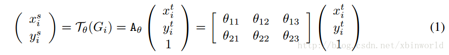
s表示source（U中的坐标），t表示target（V中的坐标）。通过仿射变换，找到目标V中的坐标点对应的source U中的坐标点。

Sampler 
作者也叫这一步Differentiable Image Sampling，是希望通过写成一种形式上可微的图像采样方法，目的是为了让整个网络保持可以端到端反向传播BP训练，用一种比较简洁的形式表示双线性插值的公式：

和最前面双线性插值的示意图含义是一样的，只是因为在图像中，相邻两个点的坐标差是1，就没有分母部分了。而循环中大部分都没用的，只取相邻的四个点作为一个grid。

所以上面 Grid generator和 Sampler是配合的，先通过V中坐标 (xtarget,ytarget) 以此找到它在U中的坐标，然后再通过双线性插值采样出真实的像素值，放到 (xtarget,ytarget) 。

基本结构与前向传播

论文中的结构图描述得不是很清楚，个人做了部分调整，如下：

DeepMind为了描述这个空间变换层，首先添加了坐标网格计算的概念，即：

对应输入源特征图像素的坐标网格——Sampling Grid，保存着 (xSource,ySource) (xSource,ySource)

对应输出源特征图像素的坐标网格——Regluar Grid  ，保存着 (xTarget,yTarget) (xTarget,yTarget)

然后，将仿射矩阵神经元组命名为定位网络 (Localisation Network)。

对于一次神经元提供参数，坐标变换计算，记为  τθ(G) τθ(G)，根据1.2，有:

τθ(Gi)=[θ11θ21θ12θ22θ13θ23]′⋅⎡⎣⎢⎢xTargetiyTargeti1⎤⎦⎥⎥=[xSourceiySourcei]wherei=1,2,3,4..,H∗W τθ(Gi)=[θ11θ12θ13θ21θ22θ23]′⋅[xiTargetyiTarget1]=[xiSourceyiSource]wherei=1,2,3,4..,H∗W

该部分对应于图中的①②，但是与论文中的图有些变化，可能是作者并没有将逆向计算的Trick搬到结构图中来。

所以你看到的仍然是Sampling Grid提供坐标给定位网络，而具体实现的时候恰好是相反的，坐标由Regluar Grid提供。

————————————————————————————————————————————————————————

Regluar Grid提供的坐标组是顺序逐行扫描坐标的序列，序列长度为  [Heght∗Width] [Heght∗Width]，即：

将2D坐标组全部1D化，根据在序列中的位置即可立即算出，在Regluar Grid中位置。

这么做的最大好处在于，无须额外存储Regluar Grid坐标 (xTarget,yTarget) (xTarget,yTarget)。

因为从输入特征图 U U数组中，按下标取出的新像素值序列，仍然是逐行扫描顺序，简单分隔一下，便得到了输出特征图 V V。

该部分对应于图中的③。

————————————————————————————————————————————————————————

(1.3)中提到了，直接简单按照 (xSource,ySource) (xSource,ySource)，从源像素数组中复制像素值是不可行的。

因为仿射变换后的 (xSource,ySource) (xSource,ySource)可以为实数，但是像素位置坐标必须是整数。

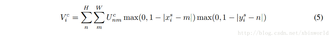
为了解决像素值缺失问题，必须进行插值。插值核函数很多，源码中选择了论文中提供的第二种插值方式——双线性插值。

(1.3)的插值式非常不优雅，DeepMind在论文利用max与abs函数，改写成一个简洁、优雅的插值等式：

Vci=∑Hn∑WmUcnmmax(0,1−|xSi−m|)max(0,1−|ySi−n|)wherei∈[1,H′W′],c∈[1,3] Vic=∑nH∑mWUnmcmax(0,1−|xiS−m|)max(0,1−|yiS−n|)wherei∈[1,H′W′],c∈[1,3]

两个  ∑ ∑ 实际上只筛出了四个邻近插值点，虽然写法简洁，但白循环很多，所以源码中选择了直接算4个点，而不是用循环筛。

该部分对应图中的④。

2.3 梯度流动与反向传播

添加空间变换层之后，梯度流动变得有趣了，如图：

The GTSRB dataset

The GTSRB dataset (German Traffic Sign Recognition Benchmark) is provided by the Institut für Neuroinformatik group here. It was published for a competition held in 2011 (results). Images are spread across 43 different types of traffic signs and contain a total of 39,209 train examples and 12,630 test ones.

We like this dataset a lot at Moodstocks: it’s lightweight, yet hard enough to test new ideas. For the record, the contest winner achieved a 99,46% top-1 accuracy thanks to a committee of 25 networks and by using a bunch of augmentations and data normalization techniques.

Spatial Transformer networks

The goal of spatial transformers [1] is to add to your base network a layer able to perform an explicit geometric transformation on an input. The parameters of the transformation are learnt thanks to the standard backpropagation algorithm, meaning there is no need for extra data or supervision.

The layer is composed of 3 elements:

• The localization network takes the original image as an input and outputs the parameters of the transformation we want to apply.
• The grid generator generates a grid of coordinates in the input image corresponding to each pixel from the output image.
• The sampler generates the output image using the grid given by the grid generator.

As an example, here is what you get after training a network whose first layer is a ST:

On the left you see the input image. In the middle you see which part of the input image is sampled. On the right you see the Spatial Transformer output image.

Results

The IDSIA guys won the contest back in 2011 with a 99.46% top-1 accuracy. We achieved a 99.61% top-1 accuracy with a much simpler pipeline:

| Pipeline | IDSIA | Moodstocks | | ------------- | --------- | ---------- | | Augmentations | Yes (i) | No | | Jittering | Yes (ii) | No | | Network | ~90M weights (iii)| ~20M weights (iv)|

• (i) 5 versions of the original dataset thanks to fancy normalization techniques
• (ii) scaling translations and rotations
• (iii) 25 networks with 3 convolutional layers and 2 fully connected layers each
• (iv) A single network with 3 convolutional layers and 2 fully connected layers + 2 spatial transformer layers

Interpretation

Given these good results, we wanted to have some insights on which kind of transformations the Spatial Transformer is learning. Since we have a Spatial Transformer at the beginning of the network we can easily visualize its impact by looking at the transformed input image.

At training time

Here the goal is to visualize how the Spatial Transformer behaves during training.

In the animation below, you can see:

• on the left the original image used as input,
• on the right the transformed image produced by the Spatial Transformer,
• on the bottom a counter that represents training steps (0 = before training, 10/10 = end of epoch 1).

Note: the white dots on the input image show the corners of the part of the image that is sampled. Same applies below.

As expected, we see that during the training, the Spatial Transformer learns to focus on the traffic sign, learning gradually to remove background.

Post-training

Here the goal is to visualize the ability of the Spatial Transformer (once trained) to produce a stable output even though the input contains geometric noise.

For the record the GTSRB dataset has been initially generated by extracting images from video sequences took while approaching a traffic sign.

The animation below shows for each image of such a sequence (on the left) the corresponding output of the Spatial Transformer (on the right).

We can see that even though there is an important variability in the input images (scale and position in the image), the output of the Spatial Transformer remains almost static.

This confirms the intuition we had on how the Spatial Transformer simplifies the task for the rest of the network: learning to only forward the interesting part of the input and removing geometric noise.

The Spatial Transformer learned these transformations in an end-to-end fashion, without any modification to the backpropagation algorithm and without any extra annotations.