Tensorflow and CNNs 使用tensorflow构建卷积神经网络

本文是我在学习cnn时看到的一个教程，觉得不错，就翻译一下。才疏学浅，如有疏漏，还请见谅。
原文：A Guide to TF Layers: Building a Convolutional Neural Network
是来自TensorFlow的开发者文档

---

TensorFlow的layers模块提供了比较高级的API，使得我们能可以很方便的构建各种神经网络。它提供的方法可以方便的添加全连接层、卷积层、激活函数以及dropout。在这个教程中，你将了解如何使用layers模块来构建用于识别MNIST数据集的卷积神经网络

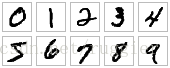
MNIST数据集包括60000张用于训练的图片和10000张用于测试的图片。每张图片一张像素为28*28的手写数字。

开始

首先构建这个TensorFlow项目的框架，创建一个名为cnn_mnist.py的文件，然后添加以下代码。

from __future__ import absolute_import
from __future__ import division
from __future__ import print_function

# Imports
import numpy as np
import tensorflow as tf

tf.logging.set_verbosity(tf.logging.INFO)

# Our application logic will be added here

if __name__ == "__main__":
    tf.app.run()

在这个教程中，我们会逐渐的添加代码已完成整个卷积神经网络的训练和测试部分。
最终完整的代码可以在github看到。

卷积神经网络简介

卷积神经网络（Convolutional neural networks, CNNS)是如今在图片分类领域最先进的方法。它通过一系列的卷积核（Convolutional Filter）从原始图片中抽取特征，然后进行分类。CNNs包含三个部分：

• 卷积层(Convolutional layers)，使用一定数量的卷积核处理原始图片。一般使用ReLU激活函数。
• 池化层(pooling layer)，对于卷积层得到的数据进行下采样以减少feature map的维度，这样可以缩短处理时间。常用的池化方法是最大池化(max pooling)。
• 全连接层(fully connected layers)，根据经过卷积层和池化层的特征进行分类。

通常来讲，CNNs是由执行特征提取的一堆卷积模块组成的。每个模块由一个卷积层和一个池层组成。最后一个卷积模块之后是一个或多个执行分类的全连接层。CNN中的最后一个Dense层包含模型中每个目标类的单个节点（模型中所有可能的类），使用softmax激活函数为每个节点生成0-1之间的值（这些值的和为1）。我们可以将每个节点对应的值看作将图片分为该类的可能性的度量。

构建分类器

使用以下CNN结构对MNIST数据集中的图像进行分类：

• Convolutional Layer #1：包含32个5x5的卷积核（抽取5x5像素子区域），使用ReLU作为激活函数。
• Pooling Layer #1： 使用2x2过滤器执行最大池化，stride为2（指定合并的区域不重叠)
• Convolutional Layer #2：包含64个5x5的卷积核，使用ReLU作为激活函数。
• Pooling Layer #1： 使用2x2过滤器执行最大池化，stride为2
• Dense Layer #1：1024个神经元， dropout regularization rate 为0.4（在训练的过程中，每个神经元都有0.4的概率被丢弃）
• Dense Layer #2 (Logits Layer): 10 个神经元, 对应着十个分类。

tf.layers模块包含创建上述三种网络层的方法：

• conv2d()。 构造一个二维卷积层。 参数：卷积核数量，卷积核大小，padding， 激活函数。
• max_pooling2d()。 使用最大池化算法构造一个池化层。参数： 过滤器大小、步幅。
• dense()。 构建一个全连接层。 参数：神经元数量、激活函数。

以上每一个方法都接受tensor作为输入，并将变换后的tensor作为输出返回。 这样可以很容易地将一个层连接到另一个层：只需将前一层的输出作为输入提供给后一层即可。

打开cnn_mnist.py 添加以下代码

def cnn_model_fn(features, labels, mode):
  """Model function for CNN."""
  # Input Layer
  input_layer = tf.reshape(features["x"], [-1, 28, 28, 1])

  # Convolutional Layer #1
  conv1 = tf.layers.conv2d(
      inputs=input_layer,
      filters=32,
      kernel_size=[5, 5],
      padding="same",
      activation=tf.nn.relu)

  # Pooling Layer #1
  pool1 = tf.layers.max_pooling2d(inputs=conv1, pool_size=[2, 2], strides=2)

  # Convolutional Layer #2 and Pooling Layer #2
  conv2 = tf.layers.conv2d(
      inputs=pool1,
      filters=64,
      kernel_size=[5, 5],
      padding="same",
      activation=tf.nn.relu)
  pool2 = tf.layers.max_pooling2d(inputs=conv2, pool_size=[2, 2], strides=2)

  # Dense Layer
  pool2_flat = tf.reshape(pool2, [-1, 7 * 7 * 64])
  dense = tf.layers.dense(inputs=pool2_flat, units=1024, activation=tf.nn.relu)
  dropout = tf.layers.dropout(
      inputs=dense, rate=0.4, training=mode == tf.estimator.ModeKeys.TRAIN)

  # Logits Layer
  logits = tf.layers.dense(inputs=dropout, units=10)

  predictions = {
      # Generate predictions (for PREDICT and EVAL mode)
      "classes": tf.argmax(input=logits, axis=1),
      # Add `softmax_tensor` to the graph. It is used for PREDICT and by the
      # `logging_hook`.
      "probabilities": tf.nn.softmax(logits, name="softmax_tensor")
  }

  if mode == tf.estimator.ModeKeys.PREDICT:
    return tf.estimator.EstimatorSpec(mode=mode, predictions=predictions)

  # Calculate Loss (for both TRAIN and EVAL modes)
  loss = tf.losses.sparse_softmax_cross_entropy(labels=labels, logits=logits)

  # Configure the Training Op (for TRAIN mode)
  if mode == tf.estimator.ModeKeys.TRAIN:
    optimizer = tf.train.GradientDescentOptimizer(learning_rate=0.001)
    train_op = optimizer.minimize(
        loss=loss,
        global_step=tf.train.get_global_step())
    return tf.estimator.EstimatorSpec(mode=mode, loss=loss, train_op=train_op)

  # Add evaluation metrics (for EVAL mode)
  eval_metric_ops = {
      "accuracy": tf.metrics.accuracy(
          labels=labels, predictions=predictions["classes"])}
  return tf.estimator.EstimatorSpec(
      mode=mode, loss=loss, eval_metric_ops=eval_metric_ops)

以下部分深入介绍用于创建每个模块的tf.layers代码，以及如何计算损失函数，配置训练操作并生成预测。

Input Layer

layers模块中的该方法用于创建适用于卷积层和池化层的输入。
参数：
- batch_size：在训练的过程中每输入batch_size个样例进行一次梯度下降。
- image_width：样例图片的宽度
- image_height：样例图片的高度
- channels：图片的通道数

这里，我们的MNIST数据集由单色的28x28像素图像组成，所以我们输入图层的期望形状是[batch_size，28,28,1]。

为了将我们的输入feature map（特征）转换成这个形状，我们可以执行下面的整形操作：

input_layer = tf.reshape(features["x"], [-1, 28, 28, 1])

要注意的是， 我们已指定batch_size大小为-1，它指定此维度应该根据features[“x”]中的输入值的大小动态计算，并保持所有其他维度的大小不变。举个例子，如果每个batch中包含五个样例，那么feature[“x”]中将包含3920个数值（每个数值表示图片中的一个像素点），input_layer的shape将会是[5, 28, 28, 1]。类似的，如果每个batch中包含一百个样例，那么feature[“x”]中将包含78400个数值，input_layer的shape将会是[100, 28, 28, 1]。

Convolutional Layer #1

在第一个卷积层包含32个5x5的卷积核，并使用ReLU作为激活函数。 我们可以使用layers模块中的conv2d()方法来创建该层，如下所示：

conv1 = tf.layers.conv2d(
    inputs=input_layer,
    filters=32,
    kernel_size=[5, 5],
    padding="same",
    activation=tf.nn.relu)

• inputs：参数指定输入张量，这里设置为为input_layer，它的shape必须为[batch_size, image_width, image_height, channels]，这里我们将input_layer连接到第一个卷积层，它的shape为[5, 28, 28, 1]。
• filters>：指定卷积核的数量

• kernel_size：制定卷积核的大小（tip:如果卷积核的宽和高相等，那么kernel_size的值可以为一个整型变量。例如这里可以写为kernel_size=5）

• padding： 参数为两个枚举值之一（不区分大小写）:same 和valid。用于决定输出张量是否和输入张量具有相同过的维度。这里，设置padding = same，意味着TensorFlow将0值添加到输入张量的边缘以保持输入张量的宽度和高度为28.（否则，28x28张量经过5x5卷积将产生24x24张量）

• activation: 用于指定激活函数

Pooling Layer #1

接下来，把刚创建的卷积层连接到第一个池化层。 我们可以使用layers模块中的max_pooling2d()方法来构建一个使用最大池化算法的池化层，指定步幅为2， 大小为2x2：

pool1 = tf.layers.max_pooling2d(inputs=conv1, pool_size=[2, 2], strides=2)

• inputs指定输入张量，shape为[batch_size，image_width，image_height，channels]。 在这里，我们的输入张量是conv1，来自第一个卷积层的输出，其shape为[batch_size，28,28,32]。
• pool_size参数指定池化层的filter的大小为[width, height]，如果宽和高相同，则可以用一个数字代替。
• strides参数指定步幅的大小。 在这里，我们设置为2，这意味着由滤波器提取的子区域应该在宽度和高度两个方向上分开2个像素（对于2x2滤波器，这意味着没有提取的区域将重叠）。 如果要为宽度和高度设置不同的跨度值，则可以指定元组或列表（例如，stride = [3，6]）。

由max_pooling2d()（pool1）生成的输出张量的形状为[batch_size，14，14，32]：2x2滤波器将宽度和高度分别减少50％。

Convolutional Layer #2 and Pooling Layer #2

和上面一样，我们可以使用conv2d()和max_pooling2d() 向CNN中添加第二个卷积层和池化层

conv2 = tf.layers.conv2d(
    inputs=pool1,
    filters=64,
    kernel_size=[5, 5],
    padding="same",
    activation=tf.nn.relu)

pool2 = tf.layers.max_pooling2d(inputs=conv2, pool_size=[2, 2], strides=2)

值得注意的是， 第二个卷积层的输入为第一个池化层的输出，输出为conv2，它的shape为[batch_size，14，14，64]，宽和高与池化层的输出相同（由于padding="same"，64是因为第二个卷积层有64个卷积核。）

第二个池化层的输入为conv2， 输出为pool2，shape为[batch_size，7, 7,64]

Dense Layer

接下来，我们想要在我们的CNN中添加一个全连接层（神经元个数为1024，激活函数为ReLU）来对卷积/池化层提取的特征进行分类。 然而，在我们连接图层之前，我们会将我们的feature map（pool2）扁平化以形成[batch_size，features]，这样我们的张量只有两个维度：

pool2_flat = tf.reshape(pool2, [-1, 7 * 7 * 64])

在上面的reshape()操作中，-1表示batch_size维度将根据输入数据中的示例数量动态计算。 每个示例都有7个（pool2的宽度）* 7（pool2的高度）* 64（pool2的通道数）个feature，所以我们希望feature能维度的值为7 * 7 * 64（共3136个）。 输出张量pool2_flat的形状为[batch_size，3136]。
接下来，我们可以使用layers模块中的dense()方法来添加全连接层，如下所示：

dense = tf.layers.dense(inputs=pool2_flat, units=1024, activation=tf.nn.relu

• inputs指定输入张量：这里将feature map扁平化后的pool2_flat作为参数。
• units参数指定神经元个数（1,024）。
• activation采用激活函数。

为了帮助改进我们的模型的结果，我们也将dropout正则化应用于我们的全连接层：

dropout = tf.layers.dropout(
    inputs=dense, rate=0.4, training=mode == tf.estimator.ModeKeys.TRAIN)

• rate: 这里设置为0.4，表示每个神经元都有0.4的概率会在训练的过程中被舍弃.
• training：采用布尔值来指定模型当前是否在训练模式下运行，只有在训练模式下，才会进行dropout

dropout 的输入张量，shape为[batch_size, 1024]

Logits Layer

最后一层是logits层，它将返回我们预测的原始值。 我们创建了一个包含10个神经元（每个目标类为0-9）的全连接层，使用线性激活函数：

logits = tf.layers.dense(inputs=dropout, units=10)

输出张量的shape为[batch_size, 10]

预测

logits层将会输出为shape为[batch_size, 10]的原始值，我们可以将这些原始值转化成一下两种格式：

• 对于每个样例的预测类别（0-9）的数字
• 样例属于每个类别的概率。

对于给定的一个样例，我们选择在logits输出张量中最大的值对应的分类作为最终的预测分类，可以通过tf.argmax来找到这个对应的分类：

tf.argmax(input=logits, axis=1)

我们可以通过使用tf.nn.softmax应用softmax从logits层中得出概率：

tf.nn.softmax(logits, name="softmax_tensor")

用字典表示预测，返回一个EstimatorSpec 对象

predictions = {
    "classes": tf.argmax(input=logits, axis=1),
    "probabilities": tf.nn.softmax(logits, name="softmax_tensor")
}
if mode == tf.estimator.ModeKeys.PREDICT:
  return tf.estimator.EstimatorSpec(mode=mode, predictions=predictions)

损失函数

对于训练和评估，我们需要定义一个损失函数来衡量模型的预测与目标类别的匹配程度。 对于像MNIST这样的多类分类问题，通常使用交叉熵作为损失度量。 以下代码计算模型在TRAIN或EVAL模式下运行时的交叉熵：

onehot_labels = tf.one_hot(indices=tf.cast(labels, tf.int32), depth=10)
loss = tf.losses.softmax_cross_entropy(
    onehot_labels=onehot_labels, logits=logits)

我们来解释一下上面的代码
label张量包含了训练样例的预测值，如[1, 9, ...]，为了计算交叉熵，我们需要将其转化成one-hot encoding

[[0, 1, 0, 0, 0, 0, 0, 0, 0, 0],
 [0, 0, 0, 0, 0, 0, 0, 0, 0, 1],
 ...]

我们使用tf.one_hot进行这种转换，tf.one_hot需要两个参数：
- indices：one-hot张量中1的位置
- depth：one-hot 张量的长度，在这里是10
下面这行代码就可以将label转化成one-hot张量，onehot_label:

onehot_labels = tf.one_hot(indices=tf.cast(labels, tf.int32), depth=10)

接下来，我们计算onehot_labels与自logits层的预测值之间的交叉熵。tf.losses.softmax_cross_entropy()将onehot_labels和logits作为参数，对logits使用softmax处理，计算交叉熵，并将我们的损失作为标量Tensor返回：

loss = tf.losses.softmax_cross_entropy(onehot_labels=onehot_labels, logits=logits)

训练

我们已经将CNN的损失定义为logits层和标签softmax的交叉熵。 接下来配置模型，在训练期间优化这个损失值。 我们将使用0.001的学习率和随机梯度下降作为优化算法：

if mode == tf.estimator.ModeKeys.TRAIN:
  optimizer = tf.train.GradientDescentOptimizer(learning_rate=0.001)
  train_op = optimizer.minimize(
      loss=loss,
      global_step=tf.train.get_global_step())
  return tf.estimator.EstimatorSpec(mode=mode, loss=loss, train_op=train_op)

评估

要在模型中添加 准确性度量，我们在EVAL模式中定义eval_metric_ops字典，如下所示：

eval_metric_ops = {
    "accuracy": tf.metrics.accuracy(
        labels=labels, predictions=predictions["classes"])}
return tf.estimator.EstimatorSpec(
    mode=mode, loss=loss, eval_metric_ops=eval_metric_ops)

---

训练及评估CNN MNIST分类器

我们已经构建好了模型，接下来进行训练和评估

加载数据

首先，加载训练和测试数据，在cnn_mnist.py中添加main()

def main(unused_argv):
    # Load training and eval data
    mnist = tf.contrib.learn.datasets.load_dataset("mnist")
    train_data = mnist.train.images # Returns np.array
    train_labels = np.asarray(mnist.train.labels, dtype=np.int32)
    eval_data = mnist.test.images # Returns np.array
    eval_labels = np.asarray(mnist.test.labels, dtype=np.int32)

我们将训练特征数据（55,000个手绘数字图像的原始像素值）和训练标签（每个图像0-9的相应值）分别存储在train_data和train_labels中。 同样，我们将评估特征数据（10,000个图像）和评估标签分别存储在eval_data和eval_labels中。

评价模型

接下来创建一个Estimator（TensorFlow的一个类，用于高级模型的训练和推导）

# Create the Estimator
mnist_classifier = tf.estimator.Estimator(
    model_fn=cnn_model_fn, model_dir="/tmp/mnist_convnet_model")

• model_fn：指定用于训练、评估和预测的模型函数;我们将之前创建的cnn_model_fn作为参数。
• model_dir：指定用于保存模型数据（检查点）的目录（这里，我们指定临时目录/ tmp / mnist_convnet_model，但可以随意更改为您选择的另一个目录）。

记录日志

由于CNNs的训练可能比较耗时，所以我们设置一些日志记录，便于跟踪进度。这里可以使用tf.train.SessionRunHook来创建一个tf.train.LoggingTensorHook，在main()中添加如下代码：

# Set up logging for predictions
  tensors_to_log = {"probabilities": "softmax_tensor"}
  logging_hook = tf.train.LoggingTensorHook(
      tensors=tensors_to_log, every_n_iter=50)

tensors_to_log是我们想要保存的张量组成的字典，每个键都是我们选择的标签，将被打印在日志输出中。相应的标签是TensorFlow图中张量的名称。在这里，probabilities可以在softmax_tensor中找到，这是我们在cnn_model_fn中生成概率时先前给出的softmax操作的名字。
然后创建LoggingTensorHook，将tensors_to_log传递给tensors。 我们设置every_n_iter = 50，它指定在每50次训练之后记录probabilities。

训练模型

现在我们准备开始训练模型，可以通过在mnist_classifier上创建train_input_fn并调用 train()来完成，在main()中添加如下代码：

# Train the model
train_input_fn = tf.estimator.inputs.numpy_input_fn(
    x={"x": train_data},
    y=train_labels,
    batch_size=100,
    num_epochs=None,
    shuffle=True)
mnist_classifier.train(
    input_fn=train_input_fn,
    steps=20000,
    hooks=[logging_hook])

在调用numpy_input_fn中，我们将训练特征数据和标签分别传递给x（作为字典）和y。
- batch_size设置为100（这意味着模型每次传入100张图片）。
-num_epochs = None意味着模型将一直训练，直到达到指定的步数
-shuffle = True， 意味着每次训练前将会打乱数据。
在调用train()中，我们设置了steps= 20000（这意味着模型将训练总计20000次）。 我们将logging_hook传递给hooks`参数，以便在训练过程中触发它。

评估模型

一旦训练完成，我们要评估我们的模型，以确定其在MNIST测试集上的准确性。 我们调用评估方法，评估我们在model_fn中的定义的eval_metric_ops参数中指定的度量。

# Evaluate the model and print results
eval_input_fn = tf.estimator.inputs.numpy_input_fn(
    x={"x": eval_data},
    y=eval_labels,
    num_epochs=1,
    shuffle=False)
eval_results = mnist_classifier.evaluate(input_fn=eval_input_fn)
print(eval_results)

运行模型

我们已经完成了模型的构建、评估等模块，现在可以运行一下模型
在训练的过程中，你应该会看到如下的日志：

INFO:tensorflow:loss = 2.36026, step = 1
INFO:tensorflow:probabilities = [[ 0.07722801  0.08618255  0.09256398, ...]]
...
INFO:tensorflow:loss = 2.13119, step = 101
INFO:tensorflow:global_step/sec: 5.44132
...
INFO:tensorflow:Loss for final step: 0.553216.

INFO:tensorflow:Restored model from /tmp/mnist_convnet_model
INFO:tensorflow:Eval steps [0,inf) for training step 20000.
INFO:tensorflow:Input iterator is exhausted.
INFO:tensorflow:Saving evaluation summary for step 20000: accuracy = 0.9733, loss = 0.0902271
{'loss': 0.090227105, 'global_step': 20000, 'accuracy': 0.97329998}

可以看到，准确率为97%

其他资源

想要了解TensorFlow中的Estimators 和使用TensorFlow实现CNNs，可以参考一下资源：

• Creating Estimators in tf.estimator 提供了关于TensorFlow中Estimator API的介绍。包括配置Estimator，编写模型函数，计算损失，定义训练操作。
• Convolutional Neural Networks 介绍了如何使用较低级的TensorFlow操作而不是Estimator构建一个MNIST CNN分类模型