


以下内容为结合李沐老师的课程和教材补充的学习笔记,以及对课后练习的一些思考,自留回顾,也供同学之人交流参考。
本节课程地址:07 自动求导【动手学深度学习v2】_哔哩哔哩_bilibili
本节教材地址:2.5. 自动微分 — 动手学深度学习 2.0.0 documentation (d2l.ai)
本节开源代码:...>d2l-zh>pytorch>chapter_preliminaries>autograd.ipynb
自动微分
正如2.4节中所说,求导是几乎所有深度学习优化算法的关键步骤。 虽然求导的计算很简单,只需要一些基本的微积分。 但对于复杂的模型,手工进行更新是一件很痛苦的事情(而且经常容易出错)。
深度学习框架通过自动计算导数,即自动微分(automatic differentiation)来加快求导。 实际中,根据设计好的模型,系统会构建一个计算图(computational graph), 来跟踪计算是哪些数据通过哪些操作组合起来产生输出。 自动微分使系统能够随后反向传播梯度。 这里,反向传播(backpropagate)意味着跟踪整个计算图,填充关于每个参数的偏导数。
一个简单的例子
作为一个演示例子,(假设我们想对函数 关于列向量
求导)。 首先,我们创建变量
x并为其分配一个初始值。
import torch

x = torch.arange(4.0)
x
输出结果:
tensor([0., 1., 2., 3.])
[在我们计算 关于
的梯度之前,需要一个地方来存储梯度。] 重要的是,我们不会在每次对一个参数求导时都分配新的内存。 因为我们经常会成千上万次地更新相同的参数,每次都分配新的内存可能很快就会将内存耗尽。 注意,一个标量函数关于向量
的梯度是向量,并且与
具有相同的形状。
x.requires_grad_(True)  # 等价于x=torch.arange(4.0,requires_grad=True)
x.grad # 默认值是None(现在计算 。)
y = 2 * torch.dot(x, x)
y
输出结果:
tensor(28., grad_fn=<MulBackward0>)
x是一个长度为4的向量,计算x和x的点积,得到了我们赋值给y的标量输出。 接下来,[通过调用反向传播函数来自动计算y关于x每个分量的梯度],并打印这些梯度。
y.backward()
x.grad
输出结果:
tensor([ 0., 4., 8., 12.])
函数 关于
的梯度应为 4
。 让我们快速验证这个梯度是否计算正确。
x.grad == 4 * x输出结果:
tensor([True, True, True, True])
[现在计算x的另一个函数。]
# 在默认情况下,PyTorch会累积梯度,我们需要清除之前的值
x.grad.zero_()
y = x.sum()
y.backward()
x.grad
输出结果:
tensor([1., 1., 1., 1.])
非标量变量的反向传播
当y不是标量时,向量y关于向量x的导数的最自然解释是一个矩阵。 对于高阶和高维的y和x,求导的结果可以是一个高阶张量。
然而,虽然这些更奇特的对象确实出现在高级机器学习中(包括[深度学习中]), 但当调用向量的反向计算时,我们通常会试图计算一批训练样本中每个组成部分的损失函数的导数。 这里(,我们的目的不是计算微分矩阵,而是单独计算批量中每个样本的偏导数之和。)
# 对非标量调用backward需要传入一个gradient参数,该参数指定微分函数关于self的梯度。
# 本例只想求偏导数的和,所以传递一个1的梯度是合适的
x.grad.zero_()
y = x * x
# 等价于y.backward(torch.ones(len(x)))
y.sum().backward()
x.grad
输出结果:
tensor([0., 2., 4., 6.])
分离计算
有时,我们希望[将某些计算移动到记录的计算图之外]。 例如,假设y是作为x的函数计算的,而z则是作为y和x的函数计算的。 想象一下,我们想计算z关于x的梯度,但由于某种原因,希望将y视为一个常数, 并且只考虑到x在y被计算后发挥的作用。
这里可以分离y来返回一个新变量u,该变量与y具有相同的值, 但丢弃计算图中如何计算y的任何信息。 换句话说,梯度不会向后流经u到x。 因此,下面的反向传播函数计算z=u*x关于x的偏导数,同时将u作为常数处理, 而不是z=x*x*x关于x的偏导数。
x.grad.zero_()
y = x * x
u = y.detach() # 将y作为常数,而不是关于x的函数
z = u * x

z.sum().backward()
x.grad == u
输出结果:
tensor([True, True, True, True])
由于记录了y的计算结果,我们可以随后在y上调用反向传播, 得到y=x*x关于的x的导数,即2*x。
x.grad.zero_()
y.sum().backward()
x.grad == 2 * x
输出结果:
tensor([True, True, True, True])
Python控制流的梯度计算
使用自动微分的一个好处是: [即使构建函数的计算图需要通过Python控制流(例如,条件、循环或任意函数调用),我们仍然可以计算得到的变量的梯度]。 在下面的代码中,while循环的迭代次数和if语句的结果都取决于输入a的值。
def f(a):
    b = a * 2
    while b.norm() < 1000:
        b = b * 2
    if b.sum() > 0:
        c = b
    else:
        c = 100 * b
    return c
让我们计算梯度。
a = torch.randn(size=(), requires_grad=True)
# 使用torch.randn()函数生成一个随机的标量张量。size=()参数指定了张量的形状为空,表示创建一个标量(0维张量)
d = f(a)
d.backward()我们现在可以分析上面定义的f函数。 请注意,它在其输入a中是分段线性的。 换言之,对于任何a,存在某个常量标量k,使得f(a)=k*a,其中k的值取决于输入a,因此可以用d/a验证梯度是否正确。
a.grad == d / a输出结果:
tensor(True)
小结
- 深度学习框架可以自动计算导数:我们首先将梯度附加到想要对其计算偏导数的变量上,然后记录目标值的计算,执行它的反向传播函数,并访问得到的梯度。
练习
1. 为什么计算二阶导数比一阶导数的开销要更大?
解:
因为二阶导数是在一阶导数的基础上计算的,故二阶导数的计算开销更大。
2. 在运行反向传播函数之后,立即再次运行它,看看会发生什么。
解:
在运行反向传播函数之后,立即再次运行它,如果不设置requires_grad=True,会报错;如果设置requires_grad=True,两次grad会叠加。
原因:PyTorch通过构建计算图求导,为节约内存,每次一轮backward计算后,计算图的内存就被释放,因此,如果需要多次backward,需要在第一次backward计算时添加retain_graph=True参数,保持计算图不被释放。
试验如下:
x = torch.arange(4.0, requires_grad=True)
y = 2 * torch.dot(x, x)
y.backward()
x.grad
输出结果:
tensor([ 0., 4., 8., 12.])
y.backward()
x.grad
---------------------------------------------------------------------------
RuntimeError Traceback (most recent call last)
Cell In[14], line 1
----> 1 y.backward()
2 x.grad
File D:\Miniconda\lib\site-packages\torch\_tensor.py:396, in Tensor.backward(self, gradient, retain_graph, create_graph, inputs)
387 if has_torch_function_unary(self):
388 return handle_torch_function(
389 Tensor.backward,
390 (self,),
(...)
394 create_graph=create_graph,
395 inputs=inputs)
--> 396 torch.autograd.backward(self, gradient, retain_graph, create_graph, inputs=inputs)
File D:\Miniconda\lib\site-packages\torch\autograd\__init__.py:173, in backward(tensors, grad_tensors, retain_graph, create_graph, grad_variables, inputs)
168 retain_graph = create_graph
170 # The reason we repeat same the comment below is that
171 # some Python versions print out the first line of a multi-line function
172 # calls in the traceback and some print out the last line
--> 173 Variable._execution_engine.run_backward( # Calls into the C++ engine to run the backward pass
174 tensors, grad_tensors_, retain_graph, create_graph, inputs,
175 allow_unreachable=True, accumulate_grad=True)
RuntimeError: Trying to backward through the graph a second time (or directly access saved tensors after they have already been freed). Saved intermediate values of the graph are freed when you call .backward() or autograd.grad(). Specify retain_graph=True if you need to backward through the graph a second time or if you need to access saved tensors after calling backward.
x = torch.arange(4.0, requires_grad=True)
y = 2 * torch.dot(x, x)
y.backward(retain_graph=True)
print(x.grad)
y.backward()
print(x.grad)
输出结果:
tensor([ 0., 4., 8., 12.])
tensor([ 0., 8., 16., 24.])
3. 在控制流的例子中,我们计算d关于a的导数,如果将变量a更改为随机向量或矩阵,会发生什么?
解:
如果直接将变量a更改为随机向量或矩阵,会报错,因为此时d为向量或矩阵,而PyTorch只能标量对张量求导。
试验如下:
def f(a):
    b = a * 2
    while b.norm() < 1000:
        b = b * 2
    if b.sum() > 0:
        c = b
    else:
        c = 100 * b
    return c
a = torch.randn((4), requires_grad=True) # a为随机向量
d = f(a)
d.backward()
---------------------------------------------------------------------------
RuntimeError Traceback (most recent call last)
Cell In[17], line 3
1 a = torch.randn((4), requires_grad=True) # a为随机向量
2 d = f(a)
----> 3 d.backward()
File D:\Miniconda\lib\site-packages\torch\_tensor.py:396, in Tensor.backward(self, gradient, retain_graph, create_graph, inputs)
387 if has_torch_function_unary(self):
388 return handle_torch_function(
389 Tensor.backward,
390 (self,),
(...)
394 create_graph=create_graph,
395 inputs=inputs)
--> 396 torch.autograd.backward(self, gradient, retain_graph, create_graph, inputs=inputs)
File D:\Miniconda\lib\site-packages\torch\autograd\__init__.py:166, in backward(tensors, grad_tensors, retain_graph, create_graph, grad_variables, inputs)
162 inputs = (inputs,) if isinstance(inputs, torch.Tensor) else \
163 tuple(inputs) if inputs is not None else tuple()
165 grad_tensors_ = _tensor_or_tensors_to_tuple(grad_tensors, len(tensors))
--> 166 grad_tensors_ = _make_grads(tensors, grad_tensors_, is_grads_batched=False)
167 if retain_graph is None:
168 retain_graph = create_graph
File D:\Miniconda\lib\site-packages\torch\autograd\__init__.py:67, in _make_grads(outputs, grads, is_grads_batched)
65 if out.requires_grad:
66 if out.numel() != 1:
---> 67 raise RuntimeError("grad can be implicitly created only for scalar outputs")
68 new_grads.append(torch.ones_like(out, memory_format=torch.preserve_format))
69 else:
RuntimeError: grad can be implicitly created only for scalar outputs
原因:

PyTorch通过构建计算图求导的过程中(上图中的反向过程),每个节点都是一个标量;当节点的因变量为向量或者矩阵时,则需构建多个计算图对该向量或矩阵中的每一个元素分别进行求导。
因此,
· 如果因变量是标量,则计算图的节点只有一个,可直接调用backward()函数;
· 如果因变量是张量,则计算图的节点有若干个,调用backward()函数需设置grad_tensors参数,即backward(torch.ones_like(d)),将因变量转换为标量再对张量求导,实际计算过程为:
先求出Jacobian矩阵中每一个元素的grad,再将Jacobian矩阵与grad_tensors参数对应的张量进行对应的点乘,如下:
设 ,则
Jacobian矩阵为:
令转换的标量为 ,令设置
grad_tensors参数引入的与 同型张量为
,则:
也即, 为
的加权和,
故所求的backward()函数结果可表示为:
因此当a为随机向量或矩阵时,代码可以修改如下:
a = torch.randn((4), requires_grad=True) # a为随机向量
d = f(a)
d.backward(torch.ones_like(d))
a.grad
输出结果:
tensor([51200., 51200., 51200., 51200.])
a = torch.randn((2, 3), requires_grad=True) # a为随机矩阵
d = f(a)
d.backward(torch.ones_like(d))
a.grad
输出结果:
tensor([[51200., 51200., 51200.],
[51200., 51200., 51200.]])
4. 重新设计一个求控制流梯度的例子,运行并分析结果。
解:试验如下:
def f(a):
    b = torch.exp(a)
    while b.norm() < 100:
        b = b * 3
    if b.sum() > 0:
        c = b
    else:
        c = 100 * b
    return c
a = torch.randn((), requires_grad=True)
d = f(a)
d.backward(torch.ones_like(d))
print(a, d, a.grad)
a.grad == d
# d = k×exp(a),求导后不变,因此,对于任意a,d的梯度都与d相等。
输出结果:
tensor(0.9349, requires_grad=True) tensor(206.3119, grad_fn=<MulBackward0>) tensor(206.3119)
tensor(True)
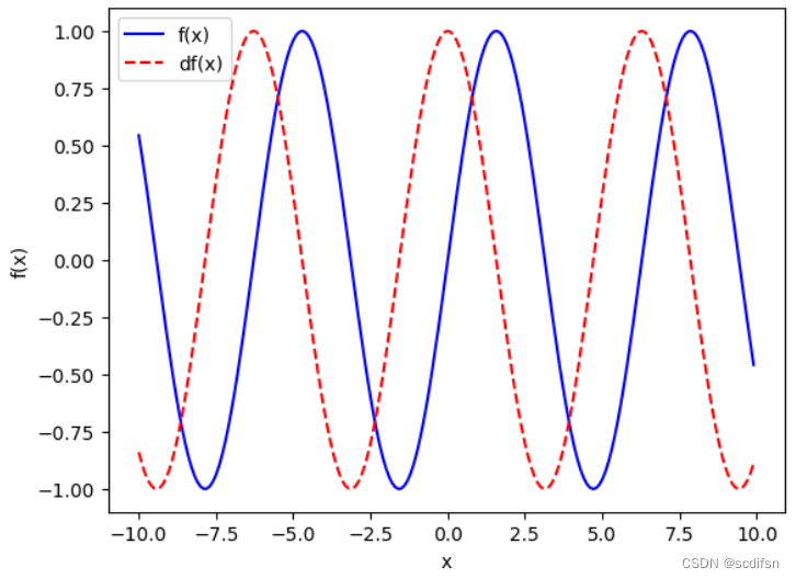
5. 使 ,绘制
和
的图像,其中后者不使用
。
解:试验如下:
import torch
import matplotlib.pyplot as plt

x = torch.arange(-10, 10, 0.1, requires_grad=True)
y = torch.sin(x)
y.backward(torch.ones_like(y))
d = x.grad
x = x.detach().numpy()
y = y.detach().numpy()
d = d.numpy()
plt.plot(x, y, 'b-', label = 'f(x)')
plt.plot(x, d, 'r--', label = 'df(x)')
plt.xlabel('x')
plt.ylabel('f(x)')
plt.legend()
plt.show()
输出结果:


 383
383


 被折叠的 条评论
为什么被折叠?
被折叠的 条评论
为什么被折叠?
 到【灌水乐园】发言


