Calculus of Variation

最新推荐文章于 2022-08-26 13:21:57 发布

shareCode

最新推荐文章于 2022-08-26 13:21:57 发布

阅读量1.8k

点赞数 1

分类专栏：数学与算法

数学与算法专栏收录该内容

4 篇文章 1 订阅

订阅专栏

From Wikipedia, the free encyclopedia

"Variational method" redirects here. For the use as an approximation method in quantum mechanics, see Variational method (quantum mechanics).

Calculus
Part of a series of articles about
Fundamental theorem Limits of functions Continuity Mean value theorem Rolle's theorem
Differential [show]
Integral [show]
Series [show]
Vector [show]
Multivariable [show]
Specialized [hide] Fractional Malliavin Stochastic Variations
v t e

Calculus of variations is a field of mathematical analysis that deals with maximizing or minimizingfunctionals, which are mappings from a set of functions to the real numbers. Functionals are often expressed as definite integrals involving functions and their derivatives. The interest is in extremalfunctions that make the functional attain a maximum or minimum value – or stationary functions – those where the rate of change of the functional is zero.

A simple example of such a problem is to find the curve of shortest length connecting two points. If there are no constraints, the solution is obviously a straight line between the points. However, if the curve is constrained to lie on a surface in space, then the solution is less obvious, and possibly many solutions may exist. Such solutions are known as geodesics. A related problem is posed by Fermat's principle: light follows the path of shortest optical length connecting two points, where the optical length depends upon the material of the medium. One corresponding concept in mechanics is the principle of least action.

Many important problems involve functions of several variables. Solutions of boundary value problems for the Laplace equation satisfy the Dirichlet principle. Plateau's problem requires finding a surface of minimal area that spans a given contour in space: a solution can often be found by dipping a frame in a solution of soap suds. Although such experiments are relatively easy to perform, their mathematical interpretation is far from simple: there may be more than one locally minimizing surface, and they may have non-trivial topology.

History[edit]

The calculus of variations may be said to begin with the brachistochrone curve problem raised by Johann Bernoulli (1696).^[1] It immediately occupied the attention of Jakob Bernoulli and the Marquis de l'Hôpital, but Leonhard Euler first elaborated the subject. His contributions began in 1733, and his Elementa Calculi Variationum gave to the science its name. Lagrange contributed extensively to the theory, and Legendre (1786) laid down a method, not entirely satisfactory, for the discrimination of maxima and minima. Isaac Newton and Gottfried Leibniz also gave some early attention to the subject.^[2] To this discrimination Vincenzo Brunacci (1810), Carl Friedrich Gauss (1829), Siméon Poisson (1831), Mikhail Ostrogradsky (1834), and Carl Jacobi (1837) have been among the contributors. An important general work is that of Sarrus (1842) which was condensed and improved byCauchy (1844). Other valuable treatises and memoirs have been written by Strauch (1849), Jellett (1850), Otto Hesse (1857), Alfred Clebsch (1858), and Carll (1885), but perhaps the most important work of the century is that of Weierstrass. His celebrated course on the theory is epoch-making, and it may be asserted that he was the first to place it on a firm and unquestionable foundation. The 20th and the 23rd Hilbert problem published in 1900 encouraged further development.^[2] In the 20th century David Hilbert, Emmy Noether, Leonida Tonelli, Henri Lebesgue and Jacques Hadamard among others made significant contributions.^[2] Marston Morse applied calculus of variations in what is now called Morse theory.^[3] Lev Pontryagin, Ralph Rockafellar and F. H. Clarke developed new mathematical tools for the calculus of variations in optimal control theory.^[3] The dynamic programmingof Richard Bellman is an alternative to the calculus of variations.^[4]^[5]^[6]

Extrema[edit]

The calculus of variations is concerned with the maxima or minima of functionals, which are collectively called extrema. A functional depends on afunction, somewhat analogous to the way a function can depend on a numerical variable, and thus a functional has been described as a function of a function. Functionals have extrema with respect to the elements $y$ of a given function space defined over a given domain. A functional $J [y]$ is said to have an extremum at the function $f$ if $ΔJ = J [y] - J [f]$ has the same sign for all $y$ in an arbitrarily small neighborhood of $f .$ ^{[Note 1]} The function $f$ is called an extremal function or extremal. The extremum $J [f]$ is called a maximum if $ΔJ \leq 0$ everywhere in an arbitrarily small neighborhood of $f,$ and a minimum if $ΔJ \geq 0$ there. For a function space of continuous functions, extrema of corresponding functionals are called weak extrema orstrong extrema, depending on whether the first derivatives of the continuous functions are respectively all continuous or not.^[8]

Both strong and weak extrema of functionals are for a space of continuous functions but weak extrema have the additional requirement that the first derivatives of the functions in the space be continuous. Thus a strong extremum is also a weak extremum, but the converse may not hold. Finding strong extrema is more difficult than finding weak extrema.^[9] An example of a necessary condition that is used for finding weak extrema is theEuler–Lagrange equation.^[10] ^{[Note 2]}

Euler–Lagrange equation[edit]

Main article: Euler–Lagrange equation

Finding the extrema of functionals is similar to finding the maxima and minima of functions. The maxima and minima of a function may be located by finding the points where its derivative vanishes (i.e., is equal to zero). The extrema of functionals may be obtained by finding functions where thefunctional derivative is equal to zero. This leads to solving the associated Euler–Lagrange equation.^{[Note 3]}

Consider the functional

J[y] = \int_{x_1}^{x_2} L(x,y(x),y'(x))\, dx \, .

where

x 1, x 2

are constants,

y (x)

is twice continuously differentiable,

y'(x) = dy / dx

L (x, y (x), y'(x))

is twice continuously differentiable with respect to its arguments

x, y, y'

If the functional $J [y]$ attains a local minimum at $f,$ and $η (x)$ is an arbitrary function that has at least one derivative and vanishes at the endpoints $x 1$ and $x 2,$ then for any number $ε$ close to 0,

J[f] \le J[f + \varepsilon \eta] \, .

The term $εη$ is called the variation of the function $f$ and is denoted by $δf .$ ^[11]

Substituting $f + εη$ for $y$ in the functional $J [y] ,$ the result is a function of $ε$ ,

\Phi(\varepsilon) = J[f+\varepsilon\eta] \, .

Since the functional $J [y]$ has a minimum for $y = f,$ the function $Φ(ε)$ has a minimum at $ε = 0$ and thus,^{[Note 4]}

\Phi'(0) \equiv \left.\frac{d\Phi}{d\varepsilon}\right|_{\varepsilon = 0} = \int_{x_1}^{x_2} \left.\frac{dL}{d\varepsilon}\right|_{\varepsilon = 0} dx = 0 \, .

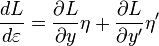
Taking the total derivative of $L [x, y, y'] ,$ where $y = f + ε η$ and $y' = f' + ε η'$ are functions of $ε$ but $x$ is not,

\frac{dL}{d\varepsilon}=\frac{\partial L}{\partial y}\frac{dy}{d\varepsilon} + \frac{\partial L}{\partial y'}\frac{dy'}{d\varepsilon}

and since $dy / dε = η$ and $dy'/ dε = η'$ ,

\frac{dL}{d\varepsilon}=\frac{\partial L}{\partial y}\eta + \frac{\partial L}{\partial y'}\eta'

Therefore,

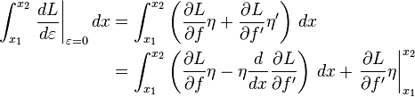
\begin{align}\int_{x_1}^{x_2} \left.\frac{dL}{d\varepsilon}\right|_{\varepsilon = 0} dx & = \int_{x_1}^{x_2} \left(\frac{\partial L}{\partial f} \eta + \frac{\partial L}{\partial f'} \eta'\right)\, dx \\ & = \int_{x_1}^{x_2} \left(\frac{\partial L}{\partial f} \eta - \eta \frac{d}{dx}\frac{\partial L}{\partial f'} \right)\, dx + \left.\frac{\partial L}{\partial f'} \eta \right|_{x_1}^{x_2}\\ \end{align}

where $L [x, y, y'] \to L [x, f, f']$ when ε = 0 and we have used integration by parts. The last term vanishes because $η = 0$ at $x 1$ and $x 2$ by definition. Also, as previously mentioned the left side of the equation is zero so that

\int_{x_1}^{x_2} \eta \left(\frac{\partial L}{\partial f} - \frac{d}{dx}\frac{\partial L}{\partial f'} \right) \, dx = 0 \, .

According to the fundamental lemma of calculus of variations, the part of the integrand in parentheses is zero, i.e.

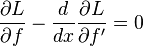
\frac{\part L}{\part f} -\frac{d}{dx} \frac{\part L}{\part f'}=0

which is called the Euler–Lagrange equation. The left hand side of this equation is called the functional derivative of $J [f]$ and is denoted $δJ / δf (x) .$

In general this gives a second-order ordinary differential equation which can be solved to obtain the extremal function $f (x) .$ The Euler–Lagrange equation is a necessary, but not sufficient, condition for an extremum $J [f]$ . A sufficient condition for a minimum is given in the section Variations and sufficient condition for a minimum.

Example[edit]

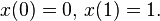
In order to illustrate this process, consider the problem of finding the extremal function $y = f (x) ,$ which is the shortest curve that connects two points $(x 1, y 1)$ and $(x 2, y 2) .$ The arc length of the curve is given by

A[y] = \int_{x_1}^{x_2} \sqrt{1 + [ y'(x) ]^2} \, dx \, ,

with

y\,'(x) = \frac{dy}{dx} \, , \ \ y_1=f(x_1) \, , \ \ y_2=f(x_2) \, .

The Euler–Lagrange equation will now be used to find the extremal function $f (x)$ that minimizes the functional $A [y] .$

\frac{\part L}{\part f} -\frac{d}{dx} \frac{\part L}{\part f'}=0

with

L = \sqrt{1 + [ f'(x) ]^2} \, .

Since $f$ does not appear explicitly in $L,$ the first term in the Euler–Lagrange equation vanishes for all $f (x)$ and thus,

\frac{d}{dx} \frac{\part L}{\part f'} = 0 \, .

Substituting for $L$ and taking the partial derivative,

\frac{d}{dx} \ \frac{ f'(x) } {\sqrt{1 + [ f'(x) ]^2}} \ = 0 \, .

Taking the derivative $d/dx$ and simplifying gives,

\frac{d^2 f}{dx^2}\ \cdot\ \frac{1}{\left[\sqrt{1+[f'(x)]^2}\ \right]^3} = 0 \, ,

and because $1+[f ' (x)] 2$ is non-zero,

\frac{d^2 f}{dx^2} = 0 \, ,

which implies that the shortest curve that connects two points $(x 1, y 1)$ and $(x 2, y 2)$ is

f(x) = m x + b \qquad \text{with} \ \ m = \frac{y_2 - y_1}{x_2 - x_1} \quad \text{and} \quad b = \frac{x_2 y_1 - x_1 y_2}{x_2 - x_1}

and we have thus found the extremal function $f (x)$ that minimizes the functional $A [y]$ so that $A [f]$ is a minimum. Note that $y = f (x)$ is the equation for a straight line, in other words, the shortest distance between two points is a straight line.^{[Note 5]}

Beltrami identity[edit]

In physics problems it frequently turns out that $\partial L / \partial x = 0$ . In that case, the Euler–Lagrange equation can be simplified to the Beltrami identity:^[12]

L-f'\frac{\part L}{\part f'}=C \, ,

where $C$ is a constant. The left hand side is the Legendre transformation of $L$ with respect to $f'$ .

Du Bois-Reymond's theorem[edit]

The discussion thus far has assumed that extremal functions possess two continuous derivatives, although the existence of the integral J requires only first derivatives of trial functions. The condition that the first variation vanishes at an extremal may be regarded as a weak form of the Euler–Lagrange equation. The theorem of Du Bois-Reymond asserts that this weak form implies the strong form. If L has continuous first and second derivatives with respect to all of its arguments, and if

\frac{\part^2 L}{(\part f')^2} \ne 0,

then $f_0$ has two continuous derivatives, and it satisfies the Euler–Lagrange equation.

Lavrentiev phenomenon[edit]

Hilbert was the first to give good conditions for the Euler–Lagrange equations to give a stationary solution. Within a convex area and a positive thrice differentiable Lagrangian the solutions are composed of a countable collection of sections that either go along the boundary or satisfy the Euler–Lagrange equations in the interior.

However Lavrentiev in 1926 showed that there are circumstances where there is no optimum solution but one can be approached arbitrarily closely by increasing numbers of sections. For instance the following:

L(t,x,x') = (x^3-t)^2 x'^6,\,

x(0)=0,\, x(1)=1.\,

Here a zig zag path gives a better solution than any smooth path and increasing the number of sections improves the solution.

Functions of several variables[edit]

Variational problems that involve multiple integrals arise in numerous applications. For example, if φ(x,y) denotes the displacement of a membrane above the domain D in the x,y plane, then its potential energy is proportional to its surface area:

U[\varphi] = \iint_D \sqrt{1 +\nabla \varphi \cdot \nabla \varphi} dx\,dy.\,

Plateau's problem consists of finding a function that minimizes the surface area while assuming prescribed values on the boundary of D; the solutions are called minimal surfaces. The Euler–Lagrange equation for this problem is nonlinear:

\varphi_{xx}(1 + \varphi_y^2) + \varphi_{yy}(1 + \varphi_x^2) - 2\varphi_x \varphi_y \varphi_{xy} = 0.\,

See Courant (1950) for details.

Dirichlet's principle[edit]

It is often sufficient to consider only small displacements of the membrane, whose energy difference from no displacement is approximated by

V[\varphi] = \frac{1}{2}\iint_D \nabla \varphi \cdot \nabla \varphi \, dx\, dy.\,

The functional V is to be minimized among all trial functions φ that assume prescribed values on the boundary of D. If u is the minimizing function and v is an arbitrary smooth function that vanishes on the boundary of D, then the first variation of $V[u + \varepsilon v]$ must vanish:

\frac{d}{d\varepsilon} V[u + \varepsilon v]|_{\varepsilon=0} = \iint_D \nabla u \cdot \nabla v \, dx\,dy = 0.\,

Provided that u has two derivatives, we may apply the divergence theorem to obtain

\iint_D \nabla \cdot (v \nabla u) \,dx\,dy = \iint_D \nabla u \cdot \nabla v + v \nabla \cdot \nabla u \,dx\,dy = \iint_C v \frac{\part u}{\part n} ds, \,

where C is the boundary of D, s is arclength along C and $\part u / \part n$ is the normal derivative of u on C. Since v vanishes on C and the first variation vanishes, the result is

\iint_D v\nabla \cdot \nabla u \,dx\,dy =0 \,

for all smooth functions v that vanish on the boundary of D. The proof for the case of one dimensional integrals may be adapted to this case to show that

\nabla \cdot \nabla u= 0 \,

in D.

The difficulty with this reasoning is the assumption that the minimizing function u must have two derivatives. Riemann argued that the existence of a smooth minimizing function was assured by the connection with the physical problem: membranes do indeed assume configurations with minimal potential energy. Riemann named this idea the Dirichlet principle in honor of his teacher Peter Gustav Lejeune Dirichlet. However Weierstrass gave an example of a variational problem with no solution: minimize

W[\varphi] = \int_{-1}^{1} (x\varphi')^2 \, dx\,

among all functions φ that satisfy $\varphi(-1)=-1$ and $\varphi(1)=1.$ $W$ can be made arbitrarily small by choosing piecewise linear functions that make a transition between −1 and 1 in a small neighborhood of the origin. However, there is no function that makes $W=0$ .^[13] Eventually it was shown that Dirichlet's principle is valid, but it requires a sophisticated application of the regularity theory for elliptic partial differential equations; see Jost and Li-Jost (1998).

Generalization to other boundary value problems[edit]

A more general expression for the potential energy of a membrane is

V[\varphi] = \iint_D \left[ \frac{1}{2} \nabla \varphi \cdot \nabla \varphi + f(x,y) \varphi \right] \, dx\,dy \, + \int_C \left[ \frac{1}{2} \sigma(s) \varphi^2 + g(s) \varphi \right] \, ds.

This corresponds to an external force density $f(x,y)$ in D, an external force $g(s)$ on the boundary C, and elastic forces with modulus $\sigma(s)$ acting on C. The function that minimizes the potential energy with no restriction on its boundary values will be denoted by u. Provided that f and gare continuous, regularity theory implies that the minimizing function u will have two derivatives. In taking the first variation, no boundary condition need be imposed on the increment v. The first variation of $V[u + \varepsilon v]$ is given by

\iint_D \left[ \nabla u \cdot \nabla v + f v \right] \, dx\, dy + \int_C \left[ \sigma u v + g v \right] \, ds =0. \,

If we apply the divergence theorem, the result is

\iint_D \left[ -v \nabla \cdot \nabla u + v f \right] \, dx \, dy + \int_C v \left[ \frac{\part u}{\part n} + \sigma u + g \right] \, ds =0. \,

If we first set v=0 on C, the boundary integral vanishes, and we conclude as before that

- \nabla \cdot \nabla u + f =0 \,

in D. Then if we allow v to assume arbitrary boundary values, this implies that u must satisfy the boundary condition

\frac{\part u}{\part n} + \sigma u + g =0, \,

on C. Note that this boundary condition is a consequence of the minimizing property of u: it is not imposed beforehand. Such conditions are callednatural boundary conditions.

The preceding reasoning is not valid if $\sigma$ vanishes identically on C. In such a case, we could allow a trial function $\varphi \equiv c$ , where c is a constant. For such a trial function,

V[c] = c\left[ \iint_D f \, dx\,dy + \int_C g ds \right].

By appropriate choice of c, V can assume any value unless the quantity inside the brackets vanishes. Therefore the variational problem is meaningless unless

\iint_D f \, dx\,dy + \int_C g \, ds =0.\,

This condition implies that net external forces on the system are in equilibrium. If these forces are in equilibrium, then the variational problem has a solution, but it is not unique, since an arbitrary constant may be added. Further details and examples are in Courant and Hilbert (1953).

Eigenvalue problems[edit]

Both one-dimensional and multi-dimensional eigenvalue problems can be formulated as variational problems.

Sturm–Liouville problems[edit]

Eigenvalue problems in several dimensions[edit]

Eigenvalue problems in higher dimensions are defined in analogy with the one-dimensional case. For example, given a domain D with boundary B in three dimensions we may define

Q[\varphi] = \iiint_D p(X) \nabla \varphi \cdot \nabla \varphi + q(X) \varphi^2 \, dx \, dy \, dz + \iint_B \sigma(S) \varphi^2 \, dS, \,

and

R[\varphi] = \iiint_D r(X) \varphi(X)^3 \, dx \, dy \, dz.\,

Let u be the function that minimizes the quotient $Q[\varphi] / R[\varphi],$ with no condition prescribed on the boundary B. The Euler–Lagrange equation satisfied by u is

-\nabla \cdot (p(X) \nabla u) + q(x) u - \lambda r(x) u=0,\,

where

\lambda = \frac{Q[u]}{R[u]}.\,

The minimizing u must also satisfy the natural boundary condition

p(S) \frac{\part u}{\part n} + \sigma(S) u =0,

on the boundary B. This result depends upon the regularity theory for elliptic partial differential equations; see Jost and Li-Jost (1998) for details. Many extensions, including completeness results, asymptotic properties of the eigenvalues and results concerning the nodes of the eigenfunctions are in Courant and Hilbert (1953).

Applications[edit]

Main article: Applications of the calculus of variations

Some applications of the calculus of variations include:

The derivation of the Catenary shape
The Brachistochrone problem
Isoperimetric problems
Geodesics on surfaces
Minimal surfaces and Plateau's problem
Optimal control

Fermat's principle[edit]

Fermat's principle states that light takes a path that (locally) minimizes the optical length between its endpoints. If the x-coordinate is chosen as the parameter along the path, and $y=f(x)$ along the path, then the optical length is given by

A[f] = \int_{x=x_0}^{x_1} n(x,f(x)) \sqrt{1 + f'(x)^2} dx, \,

where the refractive index $n(x,y)$ depends upon the material. If we try $f(x) = f_0 (x) + \varepsilon f_1 (x)$ then the first variation of A (the derivative ofA with respect to ε) is

\delta A[f_0,f_1] = \int_{x=x_0}^{x_1} \left[ \frac{ n(x,f_0) f_0'(x) f_1'(x)}{\sqrt{1 + f_0'(x)^2}} + n_y (x,f_0) f_1 \sqrt{1 + f_0'(x)^2} \right] dx.

After integration by parts of the first term within brackets, we obtain the Euler–Lagrange equation

-\frac{d}{dx} \left[\frac{ n(x,f_0) f_0'}{\sqrt{1 + f_0'^2}} \right] + n_y (x,f_0) \sqrt{1 + f_0'(x)^2} =0. \,

The light rays may be determined by integrating this equation. This formalism is used in the context of Lagrangian optics and Hamiltonian optics.

Snell's law[edit]

There is a discontinuity of the refractive index when light enters or leaves a lens. Let

n(x,y) = n_- \quad \hbox{if} \quad x<0, \,

n(x,y) = n_+ \quad \hbox{if} \quad x>0,\,

where $n_-$ and $n_+$ are constants. Then the Euler–Lagrange equation holds as before in the region where x<0 or x>0, and in fact the path is a straight line there, since the refractive index is constant. At the x=0, f must be continuous, but f' may be discontinuous. After integration by parts in the separate regions and using the Euler–Lagrange equations, the first variation takes the form

\delta A[f_0,f_1] = f_1(0)\left[ n_-\frac{f_0'(0_-)}{\sqrt{1 + f_0'(0_-)^2}} -n_+\frac{f_0'(0_+)}{\sqrt{1 + f_0'(0_+)^2}} \right].\,

The factor multiplying $n_-$ is the sine of angle of the incident ray with the x axis, and the factor multiplying $n_+$ is the sine of angle of the refracted ray with the x axis. Snell's law for refraction requires that these terms be equal. As this calculation demonstrates, Snell's law is equivalent to vanishing of the first variation of the optical path length.

Fermat's principle in three dimensions[edit]

It is expedient to use vector notation: let $X=(x_1,x_2,x_3),$ let t be a parameter, let $X(t)$ be the parametric representation of a curve C, and let $\dot X(t)$ be its tangent vector. The optical length of the curve is given by

A[C] = \int_{t=t_0}^{t_1} n(X) \sqrt{ \dot X \cdot \dot X} dt. \,

Note that this integral is invariant with respect to changes in the parametric representation of C. The Euler–Lagrange equations for a minimizing curve have the symmetric form

\frac{d}{dt} P = \sqrt{ \dot X \cdot \dot X} \nabla n, \,

where

P = \frac{n(X) \dot X}{\sqrt{\dot X \cdot \dot X} }.\,

It follows from the definition that P satisfies

P \cdot P = n(X)^2. \,

Therefore the integral may also be written as

A[C] = \int_{t=t_0}^{t_1} P \cdot \dot X \, dt.\,

This form suggests that if we can find a function ψ whose gradient is given by P, then the integral A is given by the difference of ψ at the endpoints of the interval of integration. Thus the problem of studying the curves that make the integral stationary can be related to the study of the level surfaces of ψ. In order to find such a function, we turn to the wave equation, which governs the propagation of light. This formalism is used in the context of Lagrangian optics and Hamiltonian optics.

Connection with the wave equation[edit]

The wave equation for an inhomogeneous medium is

u_{tt} = c^2 \nabla \cdot \nabla u, \,

where c is the velocity, which generally depends upon X. Wave fronts for light are characteristic surfaces for this partial differential equation: they satisfy

\varphi_t^2 = c(X)^2 \nabla \varphi \cdot \nabla \varphi. \,

We may look for solutions in the form

\varphi(t,X) = t - \psi(X). \,

In that case, ψ satisfies

\nabla \psi \cdot \nabla \psi = n^2, \,

where $n=1/c.$ According to the theory of first-order partial differential equations, if $P = \nabla \psi,$ then P satisfies

\frac{dP}{ds} = n \nabla n, \,

along a system of curves (the light rays) that are given by

\frac{dX}{ds} = P. \,

These equations for solution of a first-order partial differential equation are identical to the Euler–Lagrange equations if we make the identification

\frac{ds}{dt} = \frac{\sqrt{ \dot X \cdot \dot X} }{n}. \,

We conclude that the function ψ is the value of the minimizing integral A as a function of the upper end point. That is, when a family of minimizing curves is constructed, the values of the optical length satisfy the characteristic equation corresponding the wave equation. Hence, solving the associated partial differential equation of first order is equivalent to finding families of solutions of the variational problem. This is the essential content of the Hamilton–Jacobi theory, which applies to more general variational problems.

Action principle[edit]

Main article: Action (physics)

In classical mechanics, the action, S, is defined as the time integral of the Lagrangian, L. The Lagrangian is the difference of energies,

L = T - U, \,

where T is the kinetic energy of a mechanical system and U its potential energy. Hamilton's principle (or the action principle) states that the motion of a conservative holonomic (integrable constraints) mechanical system is such that the action integral

S = \int_{t=t_0}^{t_1} L(x, \dot x, t) dt \,

is stationary with respect to variations in the path x(t). The Euler–Lagrange equations for this system are known as Lagrange's equations:

\frac{d}{dt} \frac{\part L}{\part \dot x} = \frac{\part L}{\part x}, \,

and they are equivalent to Newton's equations of motion (for such systems).

The conjugate momenta P are defined by

p = \frac{\part L}{\part \dot x}. \,

For example, if

T = \frac{1}{2} m \dot x^2, \,

then

p = m \dot x. \,

Hamiltonian mechanics results if the conjugate momenta are introduced in place of $\dot x$ , and the Lagrangian L is replaced by the Hamiltonian H defined by

H(x, p, t) = p \,\dot x - L(x,\dot x, t).\,

The Hamiltonian is the total energy of the system: H = T + U. Analogy with Fermat's principle suggests that solutions of Lagrange's equations (the particle trajectories) may be described in terms of level surfaces of some function of X. This function is a solution of the Hamilton–Jacobi equation:

\frac{\part \psi}{\part t} + H\left(x,\frac{\part \psi}{\part x},t\right) =0.\,

Variations and sufficient condition for a minimum[edit]

Calculus of variations is concerned with variations of functionals, which are small changes in the functional's value due to small changes in the function that is its argument. The first variation^{[Note 6]} is defined as the linear part of the change in the functional, and the second variation^{[Note 7]} is defined as the quadratic part.^[14]

For example, if $J [y]$ is a functional with the function $y = y (x)$ as its argument, and there is a small change in its argument from $y$ to $y + h$ , where $h = h (x)$ is a function in the same function space as $y$ , then the corresponding change in the functional is

\Delta J[h] = J[y+h] - J[y]

. ^{[Note 8]}

The functional $J [y]$ is said to be differentiable if

\Delta J[h] = \phi [h] + \epsilon \|h\|

where $φ [h]$ is a linear functional,^{[Note 9]} $||h||$ is the norm of $h$ ,^{[Note 10]} and $ε \to 0$ as $||h|| \to 0$ . The linear functional $φ [h]$ is the first variation of $J [y]$ and is denoted by,^[18]

\delta J[h] = \phi(h)

The functional $J [y]$ is said to be twice differentiable if

\Delta J[h] = \phi_1 [h] + \phi_2 [h] + \epsilon \|h\|^2

where $φ 1 [h]$ is a linear functional (the first variation), $φ 2 [h]$ is a quadratic functional,^{[Note 11]} and $ε \to 0$ as $||h|| \to 0$ . The quadratic functional $φ 2 [h]$ is the second variation of $J [y]$ and is denoted by,^[20]

\delta^2 J[h] = \phi_2(h)

The second variation $δ 2 J [h]$ is said to be strongly positive if

\delta^2J[h] \ge k \|h\|^2

for all $h$ and for some constant $k > 0$ .^[21]

Sufficient condition for a minimum:

The functional

J [y]

has a minimum at

y = ŷ

if its first variation

δJ [h] = 0

y = ŷ

and its second variation

δ 2 J [h]

is strongly positive at

y = ŷ

. ^[22] ^{[Note 12]}

shareCode

关注

1
点赞
踩
1

收藏

觉得还不错? 一键收藏
0
评论
Calculus of Variation

From Wikipedia, the free encyclopedia"Variational method" redirects here. For the use as an approximation method in quantum mechanics, see Variational method (quantum mechanics).
复制链接

扫一扫