Tensorflow学习笔记（三）——用Tensorflow实现线性回归和逻辑回归

课程名称：CS20: Tensorflow for Deep Learning Research
视频地址：https://www.bilibili.com/video/av15898988/index_4.html#page=3
课程资源：http://web.stanford.edu/class/cs20si/index.html
参考资料：https://zhuanlan.zhihu.com/p/28924642

---

一、线性回归

线性回归是机器学习中非常简单的问题，我们用tensorflow实现一个小例子。假设出生率（$X$）和平均寿命（$Y$）之间的关系是线性的。即：$Y=wX+b$。为了求出 $w,b$，我们想使用一层的神经网络，损失函数选用平均方差。数据集下载

1.1 Tensorflow 实现

① 首先我们读取txt文件中的数据：

import utils
DATA_FILE = "D:/MachineLearning/Notes/Tensorflow/Projects/Project1/birth_life_2010.txt"
# data is a numpy array of shape (190, 2), each row is a datapoint
data,n_samples =utils.read_birth_life_data(DATA_FILE)

utils.py是github文件中已经有的，utils.read_birth_life_data(filename)是里面定义的读取数据的函数，可以自己看一下。

② 定义输入X和目标Y的占位符(placeholder)：

X = tf.placeholder(tf.float32, name='X')
Y = tf.placeholder(tf.float32, name='Y')

③ 定义需要更新和学习的参数w和b，并初始化为0

w = tf.get_variable('weight', initializer=tf.constant(0.0))
b = tf.get_variable('bia', initializer=tf.constant(0.0))

④ 构建预测模型

Y_predicted = w * X + b

⑤ 利用均方误差作为损失函数：

loss = tf.square(Y - Y_predicted, name='loss')

⑥ 利用梯度下降最小化损失函数：

optimizer = tf.train.GradientDescentOptimizer(learning_rate=0.001).minimize(loss)

⑦ 在session中执行运算：

with tf.Session() as sess:
    # Step 7: initialize the necessary variables, in this case, w and b
    sess.run(tf.global_variables_initializer())
    # Step 8: train the model
    for i in range(100):# run 100 epochs
        for x, y in data:
            # Session runs train_op to minimize loss
            sess.run(optimizer,feed_dict={X: x, Y: y})
    # Step 9: output the values of w and b
    w_out,b_out = sess.run([w,b])

在执行100个epoch以后， $w = -6.07,b = 84.93$。

当然你也可以假设其他的预测模型，例如：

$Y=wX^{2}+uX+b$

w = tf.get_variable('weights_1', initializer=tf.constant(0.0))
u = tf.get_variable('weights_2', initializer=tf.constant(0.0))
b = tf.get_variable('bias', initializer=tf.constant(0.0))

Y_predicted =w * X * X +X * u + b

最终线性回归找到的直线为：

从图中我们可以看到左下方有一些极端值，既有较低的出生率，也有较低的平均寿命，这些点在优化的过程中会让直线向左偏移，造成模型性能下降。这是因为我们选用的损失函数是均方误差，导致这些极端值占的权重过大，一种改善方法是选用Huber loss。

---

1.2 Huber Loss

Huber Loss 的定义如下：

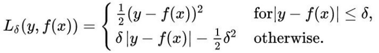
当误差比较小的时候使用均方误差，误差比较大的时候使用绝对值误差。

在实现huber loss的时候，因为tf是以图的形式来定义，所以不能使用逻辑语句，比如if等，我们可以使用TensorFlow中的条件判断语句，比如tf.where、tf.case等等。

实现Huber Loss 时我们可以选用 tf.cond ：

tf.cond(
    pred,
    true_fn=None,
    false_fn=None,
    ...)

定义Huber Loss函数如下：

def huber_loss(labels, predictions, delta=14.0):
    residual = tf.abs(labels - predictions)
    def f1(): return 0.5 * tf.square(residual)
    def f2(): return delta * residual - 0.5 * tf.square(delta)
    return tf.cond(residual < delta, f1, f2)

在执行180个epoch以后， $w = -5.87,b = 85.27$。

到底哪一个模型表现更好，我们可以设置测试集进行测试。

---

1.3 优化函数

上面我们选择了梯度下降的方法优化函数，Tensorflow还有很多优化函数可供选择：

tf.train..Optimizer 
tf.train.GradientDescentOptimizer
tf.train.AdadeltaOptimizer
tf.train.AdagradOptimizer
tf.train.AdagradDAOptimizer
tf.train.MomentumOptimizer
tf.train.AdamOptimizer
tf.train.FtrlOptimizer
tf.train.ProximalGradientDescentOptimizer
tf.train.ProximalAdagradOptimizer
tf.train.RMSPropOptimizer

---

二、MNIST逻辑回归

MNIST是手写数字数据集，里面的图像如下图所示：

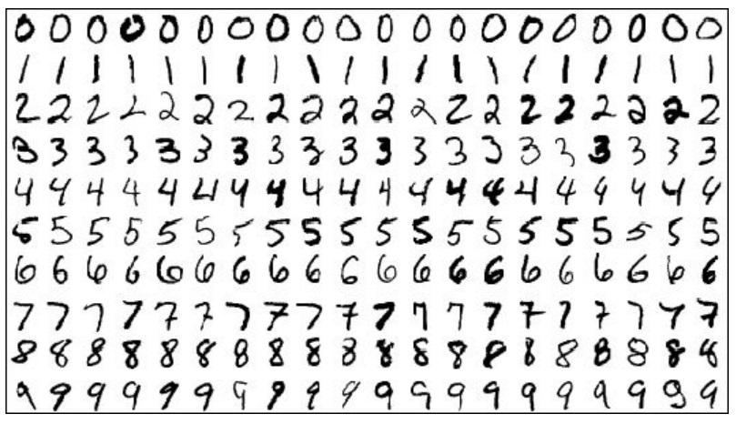
没一张图是 $28\times 28$ 像素，你可以将每一张图伸展为 784大小的向量，每一个对应一个标签——0~9中的一个数字。

2.1 Tensorflow实现

TF Learn中内置了一个脚本可以读取MNIST数据集：

from tensorflow.examples.tutorials.mnist import input_data
mnist = input_data.read_data_sets('data/mnist', one_hot=True)

接着定义占位符(placeholder)和权重参数

x = tf.placeholder(tf.float32, shape=[None, 784], name='image')
y = tf.placeholder(tf.int32, shape=[None, 10], name='label')

w = tf.get_variable('weight', shape=[784, 10], initializer=tf.truncated_normal_initializer())
b = tf.get_variable('bias', shape=[10], initializer=tf.zeros_initializer())

输入数据的shape=[None, 784]表示第一维接受任何长度的输入，第二维等于784是因为28x28=784。权重w使用均值为0,方差为1的正态分布，偏置b初始化为0。

然后定义预测结果、loss和优化函数

logits = tf.matmul(x, w) + b
entropy = tf.nn.softmax_cross_entropy_with_logits(labels=y, logits=logits)
loss = tf.reduce_mean(entropy, axis=0)
optimizer = tf.train.GradientDescentOptimizer(learning_rate=0.01).minimize(loss)

使用tf.matmul做矩阵乘法，然后使用分类问题的loss函数交叉熵，最后将一个batch中的loss求均值，对其使用随机梯度下降法。

因为数据集中有测试集，所以可以在测试集上验证其准确率

preds = tf.nn.softmax(logits)
correct_preds = tf.equal(tf.argmax(preds, 1), tf.argmax(y, 1))
accuracy = tf.reduce_sum(tf.cast(correct_preds, tf.float32), axis=0)

首先对输出结果进行softmax得到概率分布，然后使用tf.argmax得到预测的label，使用tf.equal得到预测的label和实际的label相同的个数，这是一个长为batch的0-1向量，然后使用tf.reduce_sum得到正确的总数。

最后在session中运算

with tf.Session() as sess:
    writer = tf.summary.FileWriter('./logistic_log', sess.graph)
    start_time = time.time()
    sess.run(tf.global_variables_initializer())
    n_batches = int(mnist.train.num_examples / batch_size)
    for i in range(n_epochs):  # train the model n_epochs times =10
        total_loss = 0
        for _ in range(n_batches):
            X_batch, Y_batch = mnist.train.next_batch(batch_size)
            _, loss_batch = sess.run(
                [optimizer, loss], feed_dict={x: X_batch,
                                              y: Y_batch})
            total_loss += loss_batch
        print('Average loss epoch {0}: {1}'.format(i, total_loss / n_batches))

    print('Total time: {0} seconds'.format(time.time() - start_time))

    print('Optimization Finished!')  # should be around 0.35 after 25 epochs

    # test the model
    n_batches = int(mnist.test.num_examples / batch_size) # batch_size=128
    total_correct_preds = 0

    for i in range(n_batches):
        X_batch, Y_batch = mnist.test.next_batch(batch_size)
        accuracy_batch = sess.run(accuracy, feed_dict={x: X_batch, y: Y_batch})
        total_correct_preds += accuracy_batch

    print('Accuracy {0}'.format(total_correct_preds / mnist.test.num_examples))