CS231n课程学习笔记（三）——Softmax分类器的实现

翻译笔记：https://zhuanlan.zhihu.com/p/21930884?refer=intelligentuni
作业讲解视频地址：http://www.mooc.ai/course/364/learn#lesson/2118
参考资料：http://blog.csdn.net/pjia_1008/article/details/66972060

---

作业讲解

求损失Loss

• 线性模型：$y=Wx$

• Softmax：$\displaystyle S_{i}=\frac{e^{y_{i}}}{\sum_{j}e^{y_{j}}}$

• cross-entropy Loss：$\displaystyle -\sum_{i}\mathrm{label}_{i}\log S_{i}$

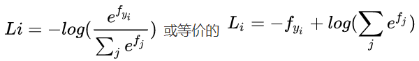
• $\mathrm{label}_{i}$是one-hot类型的，所以 $\mathrm{loss}=-\log S_{i}=-y_{i}+\log\sum_{j}e^{\hat{y}_{j}}$

  scores = X.dot(W)
  correct_class_score = scores[np.arange(num_train),y].reshape(num_train,1)
  exp_sum = np.sum(np.exp(scores),axis=1).reshape(num_train,1)
  loss += np.sum(np.log(exp_sum) - correct_class_score)
  loss /= num_train
  loss += 0.5 * reg * np.sum(W * W)

求梯度dW

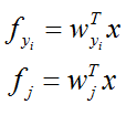
• Loss：$L_{i}=-w_{i}x_{i}+\log\sum_{j}e^{w_{j}x_{j}}$

• 对W求导：

$\left\{\begin{array}{aligned} \displaystyle dW=(-1+\frac{e^{\hat{y}_{j}}}{\sum_{j}e^{\hat{y}_{j}}})x_{i}&&j=i\\ \displaystyle dW=\frac{e^{\hat{y}_{j}}}{\sum_{j}e^{\hat{y}_{j}}}x_{i}&&j\neq i \end{array}\right.$

  margin = np.exp(scores) / exp_sum
  margin[np.arange(num_train),y] += -1
  dW = X.T.dot(margin)
  dW /= num_train
  dW += reg * W

求导具体过程：
Loss计算公式：

梯度【参考这里】：
Softmax与SVM，只是换了个损失函数，求导的思想类同，也需要分两种情况 j==$y_{i}$ 和 j!=$y_{i}$ , Softmax损失函数和求导步骤公式如下：
具体看一下这个损失函数，这里的 f 对应着scores：

所以，这里要运用链式法则，对梯度求偏导一共有两层：

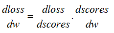
$\displaystyle\frac{\mathrm{d} scores}{\mathrm{d} w}$ 比较简单，主要解释 $\displaystyle\frac{\mathrm{d} loss}{\mathrm{d} scores}$：

j!=$y_{i}$ 针对错误项分母进行求偏导：

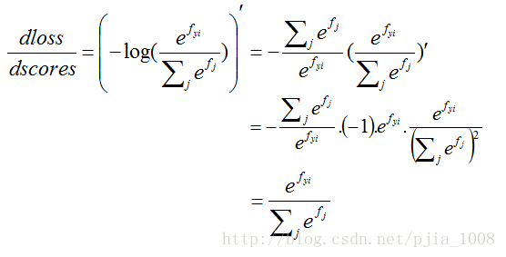
j==$y_{i}$ 针对分子进行求偏导：

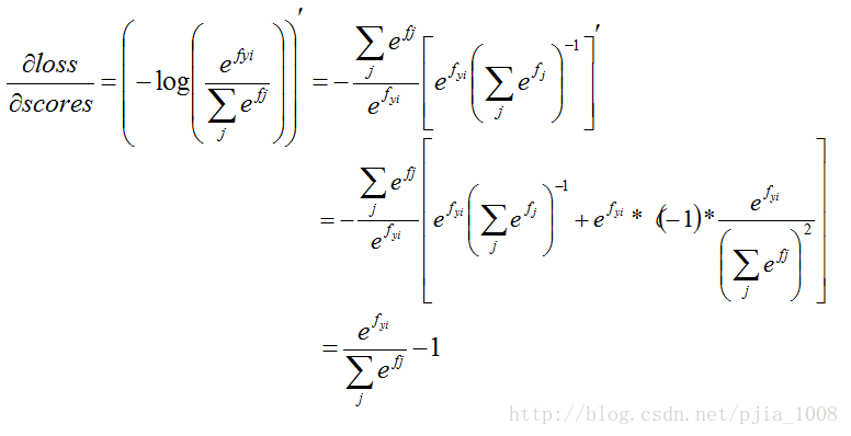
$\displaystyle\frac{\mathrm{d} loss}{\mathrm{d} scores}$到这里就完成了，再继续求$\displaystyle\frac{\mathrm{d} scores}{\mathrm{d} w}=x$,最终再乘上$\displaystyle\frac{\mathrm{d} loss}{\mathrm{d} scores}$就完成了softmax的梯度求导了！

---

SVM与Softmax分类器的比较

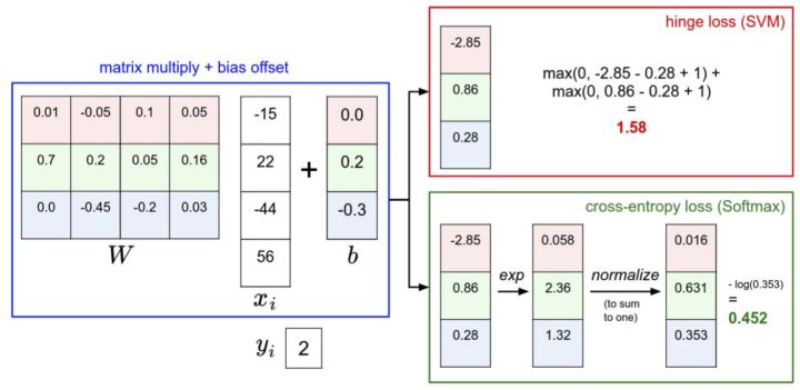
对于学习过二元逻辑回归分类器的读者来说，Softmax分类器就可以理解为逻辑回归分类器面对多个分类的一般化归纳。SVM将输出 $f(x_{i},W)$ 作为每个分类的评分（因为无定标，所以难以直接解释）。与SVM不同，Softmax的输出（归一化的分类概率）更加直观，并且从概率上可以解释，这一点后文会讨论。在Softmax分类器中，函数映射 $f(x_{i};W)=Wx_{i}$ 保持不变，但将这些评分值视为每个分类的未归一化的对数概率，并且将折叶损失（hinge loss）替换为交叉熵损失（cross-entropy loss）。公式如下：

在上式中，使用 $f_{j}$ 来表示分类评分向量 $f$ 中的第 $j$ 个元素。和之前一样，整个数据集的损失值是数据集中所有样本数据的损失值 $L_{i}$ 的均值与正则化损失$R(W)$ 之和。其中函数 $f_{j}(z)=\frac{e^{z_{j}}}{\sum_ke^{z_{k}}}$ 被称作softmax 函数：其输入值是一个向量，向量中元素为任意实数的评分值（z中的），函数对其进行压缩，输出一个向量，其中每个元素值在 $0$ 到 $1$ 之间，且所有元素之和为 1 <script type="math/tex" id="MathJax-Element-27">1</script>。

下图有助于区分这 Softmax和SVM这两种分类器：

总体代码展示

打开softmax.ipynb：

import random
import numpy as np
from cs231n.data_utils import load_CIFAR10
import matplotlib.pyplot as plt
%matplotlib inline
plt.rcParams['figure.figsize'] = (10.0, 8.0) # set default size of plots
plt.rcParams['image.interpolation'] = 'nearest'
plt.rcParams['image.cmap'] = 'gray'

加载数据并预处理

def get_CIFAR10_data(num_training=49000, num_validation=1000, num_test=1000, num_dev=500):
  """
  Load the CIFAR-10 dataset from disk and perform preprocessing to prepare
  it for the linear classifier. These are the same steps as we used for the
  SVM, but condensed to a single function.  
  """
  # Load the raw CIFAR-10 data
  cifar10_dir = 'cs231n/datasets/cifar-10-batches-py'
  X_train, y_train, X_test, y_test = load_CIFAR10(cifar10_dir)

  # subsample the data
  mask = range(num_training, num_training + num_validation)
  X_val = X_train[mask]
  y_val = y_train[mask]
  mask = range(num_training)
  X_train = X_train[mask]
  y_train = y_train[mask]
  mask = range(num_test)
  X_test = X_test[mask]
  y_test = y_test[mask]
  mask = np.random.choice(num_training, num_dev, replace=False)
  X_dev = X_train[mask]
  y_dev = y_train[mask]

  # Preprocessing: reshape the image data into rows
  X_train = np.reshape(X_train, (X_train.shape[0], -1))
  X_val = np.reshape(X_val, (X_val.shape[0], -1))
  X_test = np.reshape(X_test, (X_test.shape[0], -1))
  X_dev = np.reshape(X_dev, (X_dev.shape[0], -1))

  # Normalize the data: subtract the mean image
  mean_image = np.mean(X_train, axis = 0)
  X_train -= mean_image
  X_val -= mean_image
  X_test -= mean_image
  X_dev -= mean_image

  # add bias dimension and transform into columns
  X_train = np.hstack([X_train, np.ones((X_train.shape[0], 1))])
  X_val = np.hstack([X_val, np.ones((X_val.shape[0], 1))])
  X_test = np.hstack([X_test, np.ones((X_test.shape[0], 1))])
  X_dev = np.hstack([X_dev, np.ones((X_dev.shape[0], 1))])

  return X_train, y_train, X_val, y_val, X_test, y_test, X_dev, y_dev


# Invoke the above function to get our data.
X_train, y_train, X_val, y_val, X_test, y_test, X_dev, y_dev = get_CIFAR10_data()
print ('Train data shape: ', X_train.shape)
print ('Train labels shape: ', y_train.shape)
print ('Validation data shape: ', X_val.shape)
print ('Validation labels shape: ', y_val.shape)
print ('Test data shape: ', X_test.shape)
print ('Test labels shape: ', y_test.shape)
print ('dev data shape: ', X_dev.shape)
print ('dev labels shape: ', y_dev.shape)

OUTPUT：
Train data shape: (49000, 3073)
Train labels shape: (49000,)
Validation data shape: (1000, 3073)
Validation labels shape: (1000,)
Test data shape: (1000, 3073)
Test labels shape: (1000,)
dev data shape: (500, 3073)
dev labels shape: (500,)

Softmax分类器的实现

打开cs231n\classifiers文件夹中的 softmax.py 完成SVM的实现代码。

方法一：

import numpy as np

def softmax_loss_naive(W, X, y, reg):

  # Initialize the loss and gradient to zero.
  loss = 0.0
  dW = np.zeros_like(W)

  num_classes = W.shape[1]
  num_train = X.shape[0]
  for i in range(num_train):
      scores = X[i].dot(W)
      correct_class = y[i]
      exp_scores = np.zeros_like(scores)
      row_sum = 0
      for j in range(num_classes):
          exp_scores[j] = np.exp(scores[j])
          row_sum += exp_scores[j]
      loss += -np.log(exp_scores[correct_class]/row_sum)
      #compute dW loops:
      for k in range(num_classes):
        if k != correct_class:
          dW[:,k] += exp_scores[k] / row_sum * X[i]
        else:
          dW[:,k] += (exp_scores[correct_class]/row_sum - 1) * X[i]
  loss /= num_train
  reg_loss = 0.5 * reg * np.sum(W**2)
  loss += reg_loss
  dW /= num_train
  dW += reg * W

  return loss, dW

方法二 矢量化：

def softmax_loss_vectorized(W, X, y, reg):

  # Initialize the loss and gradient to zero.
  loss = 0.0
  dW = np.zeros_like(W)

  num_train = X.shape[0]
  scores = X.dot(W)
  correct_class_score = scores[np.arange(num_train),y].reshape(num_train,1)
  exp_sum = np.sum(np.exp(scores),axis=1).reshape(num_train,1)
  loss += np.sum(np.log(exp_sum) - correct_class_score)
  loss /= num_train
  loss += 0.5 * reg * np.sum(W * W)

  #compute gradient
  margin = np.exp(scores) / exp_sum
  margin[np.arange(num_train),y] += -1
  dW = X.T.dot(margin)
  dW /= num_train
  dW += reg * W

  return loss, dW

梯度检查

返回softmax.ipynb

# Complete the implementation of softmax_loss_naive and implement a (naive)
# version of the gradient that uses nested loops.
loss, grad = softmax_loss_naive(W, X_dev, y_dev, 0.0)

# As we did for the SVM, use numeric gradient checking as a debugging tool.
# The numeric gradient should be close to the analytic gradient.
from cs231n.gradient_check import grad_check_sparse
f = lambda w: softmax_loss_naive(w, X_dev, y_dev, 0.0)[0]
grad_numerical = grad_check_sparse(f, W, grad, 10)

# similar to SVM case, do another gradient check with regularization
loss, grad = softmax_loss_naive(W, X_dev, y_dev, 1e2)
f = lambda w: softmax_loss_naive(w, X_dev, y_dev, 1e2)[0]
grad_numerical = grad_check_sparse(f, W, grad, 10)

其中，梯度检查函数为：

def grad_check_sparse(f, x, analytic_grad, num_checks=10, h=1e-5):
  """
  sample a few random elements and only return numerical
  in this dimensions.
  """

  for i in range(num_checks):
    ix = tuple([randrange(m) for m in x.shape])

    oldval = x[ix]
    x[ix] = oldval + h # increment by h
    fxph = f(x) # evaluate f(x + h)
    x[ix] = oldval - h # increment by h
    fxmh = f(x) # evaluate f(x - h)
    x[ix] = oldval # reset

    grad_numerical = (fxph - fxmh) / (2 * h)
    grad_analytic = analytic_grad[ix]
    rel_error = abs(grad_numerical - grad_analytic) / (abs(grad_numerical) + abs(grad_analytic))
    print ('numerical: %f analytic: %f, relative error: %e' % (grad_numerical, grad_analytic, rel_error))

计算loss和梯度

tic = time.time()
loss_naive, grad_naive = softmax_loss_naive(W, X_dev, y_dev, 0.00001)
toc = time.time()
print ('naive loss: %e computed in %fs' % (loss_naive, toc - tic))

from cs231n.classifiers.softmax import softmax_loss_vectorized
tic = time.time()
loss_vectorized, grad_vectorized = softmax_loss_vectorized(W, X_dev, y_dev, 0.00001)
toc = time.time()
print ('vectorized loss: %e computed in %fs' % (loss_vectorized, toc - tic))

# As we did for the SVM, we use the Frobenius norm to compare the two versions
# of the gradient.
grad_difference = np.linalg.norm(grad_naive - grad_vectorized, ord='fro')
print ('Loss difference: %f' % np.abs(loss_naive - loss_vectorized))
print ('Gradient difference: %f' % grad_difference)

OUTPUT： naive loss: 2.371882e+00 computed in 0.189139s
vectorized loss: 2.371882e+00 computed in 0.026646s
Loss difference: 0.000000
Gradient difference: 0.000000

随机梯度下降

与SVM一样，在linear_classifier.py 文件中实现SGD函数

预测准确度

与SVM一样，在linear_classifier.py 文件中实现【predict】函数

利用交叉验证集调整超参数

from cs231n.classifiers import Softmax
results = {}
best_val = -1
best_softmax = None
learning_rates = [1e-7, 5e-7]
regularization_strengths = [5e4, 1e8]

################################################################################
# TODO:                                                                        #
# Use the validation set to set the learning rate and regularization strength. #
# This should be identical to the validation that you did for the SVM; save    #
# the best trained softmax classifer in best_softmax.                          #
################################################################################
iters = 2000
for lr in learning_rates:
    for rs in regularization_strengths:
        softmax = Softmax()
        softmax.train(X_train, y_train, learning_rate=lr, reg=rs, num_iters=iters)

        y_train_pred = softmax.predict(X_train)
        acc_train = np.mean(y_train == y_train_pred)
        y_val_pred = softmax.predict(X_val)
        acc_val = np.mean(y_val == y_val_pred)

        results[(lr, rs)] = (acc_train, acc_val)

        if best_val < acc_val:
            best_val = acc_val
            best_softmax = softmax
################################################################################
#                              END OF YOUR CODE                                #
################################################################################

# Print out results.
for lr, reg in sorted(results):
    train_accuracy, val_accuracy = results[(lr, reg)]
    print ('lr %e reg %e train accuracy: %f val accuracy: %f' % (
                lr, reg, train_accuracy, val_accuracy))

print ('best validation accuracy achieved during cross-validation: %f' % best_val)

OUTPUT：
lr 1.000000e-07 reg 5.000000e+04 train accuracy: 0.326796 val accuracy: 0.343000
lr 1.000000e-07 reg 1.000000e+08 train accuracy: 0.100265 val accuracy: 0.087000
lr 5.000000e-07 reg 5.000000e+04 train accuracy: 0.331020 val accuracy: 0.355000
lr 5.000000e-07 reg 1.000000e+08 train accuracy: 0.100265 val accuracy: 0.087000
best validation accuracy achieved during cross-validation: 0.355000

在测试集上验证

# evaluate on test set
# Evaluate the best softmax on test set
y_test_pred = best_softmax.predict(X_test)
test_accuracy = np.mean(y_test == y_test_pred)
print ('softmax on raw pixels final test set accuracy: %f' % (test_accuracy, ))

OUTPUT： softmax on raw pixels final test set accuracy: 0.339000

# Visualize the learned weights for each class
w = best_softmax.W[:-1,:] # strip out the bias
w = w.reshape(32, 32, 3, 10)

w_min, w_max = np.min(w), np.max(w)

classes = ['plane', 'car', 'bird', 'cat', 'deer', 'dog', 'frog', 'horse', 'ship', 'truck']
for i in range(10):
  plt.subplot(2, 5, i + 1)

  # Rescale the weights to be between 0 and 255
  wimg = 255.0 * (w[:, :, :, i].squeeze() - w_min) / (w_max - w_min)
  plt.imshow(wimg.astype('uint8'))
  plt.axis('off')
  plt.title(classes[i])

OUTPUT：