深度学习8：YOLOv5-C3模块实现

原创已于 2025-12-19 22:16:40 修改 · 446 阅读

16 ·

CC 4.0 BY-SA版权

文章标签：

#深度学习 #YOLO #人工智能

于 2025-12-19 21:58:14 首次发布

深度学习专栏收录该内容

7 篇文章

订阅专栏

🍨 本文为🔗365天深度学习训练营中的学习记录博客
🍖 原作者：K同学啊

目录

一、前期准备

1.设置GPU

2.导入数据

3.划分数据集

二、搭建包含C3模块的模型

1. 搭建模型

2.查看模型详情

三、训练模型

1. 编写训练函数

2. 编写测试函数

3. 正式训练

四、结果可视化

1. Loss与Accuracy图

2. 模型评估

一、前期准备

1.设置GPU

import sys
sys.path.append(r'D:\Software\PyTorch') ## 指向安装 PyTorch 的目录
import torch
import torch.nn as nn
import torchvision.transforms as transforms
import torchvision
from torchvision import transforms, datasets
import os,PIL,pathlib,warnings
 
warnings.filterwarnings("ignore")             #忽略警告信息
 
device = torch.device("cuda" if torch.cuda.is_available() else "cpu")
device

2.导入数据

import os,PIL,random,pathlib

data_dir = '文件路径/'
data_dir = pathlib.Path(data_dir)

data_paths  = list(data_dir.glob('*'))
classeNames = [str(path).split("\\")[7] for path in data_paths]
classeNames

['cloudy', 'rain', 'shine', 'sunrise']

# 关于transforms.Compose的更多介绍可以参考：https://blog.csdn.net/qq_38251616/article/details/124878863
train_transforms = transforms.Compose([
    transforms.Resize([224, 224]),  # 将输入图片resize成统一尺寸
    # transforms.RandomHorizontalFlip(), # 随机水平翻转
    transforms.ToTensor(),          # 将PIL Image或numpy.ndarray转换为tensor，并归一化到[0,1]之间
    transforms.Normalize(           # 标准化处理-->转换为标准正太分布（高斯分布），使模型更容易收敛
        mean=[0.485, 0.456, 0.406], 
        std=[0.229, 0.224, 0.225])  # 其中 mean=[0.485,0.456,0.406]与std=[0.229,0.224,0.225] 从数据集中随机抽样计算得到的。
])

test_transform = transforms.Compose([
    transforms.Resize([224, 224]),  # 将输入图片resize成统一尺寸
    transforms.ToTensor(),          # 将PIL Image或numpy.ndarray转换为tensor，并归一化到[0,1]之间
    transforms.Normalize(           # 标准化处理-->转换为标准正太分布（高斯分布），使模型更容易收敛
        mean=[0.485, 0.456, 0.406], 
        std=[0.229, 0.224, 0.225])  # 其中 mean=[0.485,0.456,0.406]与std=[0.229,0.224,0.225] 从数据集中随机抽样计算得到的。
])

total_data = datasets.ImageFolder("文件路径/",transform=train_transforms)
total_data

Dataset ImageFolder
    Number of datapoints: 1125
    Root location: 文件路径/
    StandardTransform
Transform: Compose(
               Resize(size=[224, 224], interpolation=bilinear, max_size=None, antialias=True)
               ToTensor()
               Normalize(mean=[0.485, 0.456, 0.406], std=[0.229, 0.224, 0.225])
           )

total_data.class_to_idx

{'cloudy': 0, 'rain': 1, 'shine': 2, 'sunrise': 3}

3.划分数据集

train_size = int(0.8 * len(total_data))
test_size  = len(total_data) - train_size
train_dataset, test_dataset = torch.utils.data.random_split(total_data, [train_size, test_size])
train_dataset, test_dataset

batch_size = 4
train_dl = torch.utils.data.DataLoader(train_dataset,
                                           batch_size=batch_size,
                                           shuffle=True,
                                           num_workers=1)
test_dl = torch.utils.data.DataLoader(test_dataset,
                                          batch_size=batch_size,
                                          shuffle=True,
                                          num_workers=1)
for X, y in test_dl:
    print("Shape of X [N, C, H, W]: ", X.shape)
    print("Shape of y: ", y.shape, y.dtype)
    break

(<torch.utils.data.dataset.Subset at 0x22479dc9a90>,
 <torch.utils.data.dataset.Subset at 0x2247a3d8cd0>)

Shape of X [N, C, H, W]:  torch.Size([4, 3, 224, 224])
Shape of y:  torch.Size([4]) torch.int64

二、搭建包含C3模块的模型

1. 搭建模型

import torch.nn.functional as F

def autopad(k, p=None):  # kernel, padding
    # Pad to 'same'
    if p is None:
        p = k // 2 if isinstance(k, int) else [x // 2 for x in k]  # auto-pad
    return p

class Conv(nn.Module):
    # Standard convolution
    def __init__(self, c1, c2, k=1, s=1, p=None, g=1, act=True):  # ch_in, ch_out, kernel, stride, padding, groups
        super().__init__()
        self.conv = nn.Conv2d(c1, c2, k, s, autopad(k, p), groups=g, bias=False)
        self.bn = nn.BatchNorm2d(c2)
        self.act = nn.SiLU() if act is True else (act if isinstance(act, nn.Module) else nn.Identity())

    def forward(self, x):
        return self.act(self.bn(self.conv(x)))

class Bottleneck(nn.Module):
    # Standard bottleneck
    def __init__(self, c1, c2, shortcut=True, g=1, e=0.5):  # ch_in, ch_out, shortcut, groups, expansion
        super().__init__()
        c_ = int(c2 * e)  # hidden channels
        self.cv1 = Conv(c1, c_, 1, 1)
        self.cv2 = Conv(c_, c2, 3, 1, g=g)
        self.add = shortcut and c1 == c2

    def forward(self, x):
        return x + self.cv2(self.cv1(x)) if self.add else self.cv2(self.cv1(x))

class C3(nn.Module):
    # CSP Bottleneck with 3 convolutions
    def __init__(self, c1, c2, n=1, shortcut=True, g=1, e=0.5):  # ch_in, ch_out, number, shortcut, groups, expansion
        super().__init__()
        c_ = int(c2 * e)  # hidden channels
        self.cv1 = Conv(c1, c_, 1, 1)
        self.cv2 = Conv(c1, c_, 1, 1)
        self.cv3 = Conv(2 * c_, c2, 1)  # act=FReLU(c2)
        self.m = nn.Sequential(*(Bottleneck(c_, c_, shortcut, g, e=1.0) for _ in range(n)))

    def forward(self, x):
        return self.cv3(torch.cat((self.m(self.cv1(x)), self.cv2(x)), dim=1))

class model_K(nn.Module):
    def __init__(self):
        super(model_K, self).__init__()
        
        # 卷积模块
        self.Conv = Conv(3, 32, 3, 2) 
        
        # C3模块1
        self.C3_1 = C3(32, 64, 3, 2)
        
        # 全连接网络层，用于分类
        self.classifier = nn.Sequential(
            nn.Linear(in_features=802816, out_features=100),
            nn.ReLU(),
            nn.Linear(in_features=100, out_features=4)
        )
        
    def forward(self, x):
        x = self.Conv(x)
        x = self.C3_1(x)
        x = torch.flatten(x, start_dim=1)
        x = self.classifier(x)

        return x

device = "cuda" if torch.cuda.is_available() else "cpu"
print("Using {} device".format(device))
    
model = model_K().to(device)
model

Using cpu device

model_K(
  (Conv): Conv(
    (conv): Conv2d(3, 32, kernel_size=(3, 3), stride=(2, 2), padding=(1, 1), bias=False)
    (bn): BatchNorm2d(32, eps=1e-05, momentum=0.1, affine=True, track_running_stats=True)
    (act): SiLU()
  )
  (C3_1): C3(
    (cv1): Conv(
      (conv): Conv2d(32, 32, kernel_size=(1, 1), stride=(1, 1), bias=False)
      (bn): BatchNorm2d(32, eps=1e-05, momentum=0.1, affine=True, track_running_stats=True)
      (act): SiLU()
    )
    (cv2): Conv(
      (conv): Conv2d(32, 32, kernel_size=(1, 1), stride=(1, 1), bias=False)
      (bn): BatchNorm2d(32, eps=1e-05, momentum=0.1, affine=True, track_running_stats=True)
      (act): SiLU()
    )
    (cv3): Conv(
      (conv): Conv2d(64, 64, kernel_size=(1, 1), stride=(1, 1), bias=False)
      (bn): BatchNorm2d(64, eps=1e-05, momentum=0.1, affine=True, track_running_stats=True)
      (act): SiLU()
    )
    (m): Sequential(
      (0): Bottleneck(
        (cv1): Conv(
          (conv): Conv2d(32, 32, kernel_size=(1, 1), stride=(1, 1), bias=False)
          (bn): BatchNorm2d(32, eps=1e-05, momentum=0.1, affine=True, track_running_stats=True)
          (act): SiLU()
        )
        (cv2): Conv(
          (conv): Conv2d(32, 32, kernel_size=(3, 3), stride=(1, 1), padding=(1, 1), bias=False)
          (bn): BatchNorm2d(32, eps=1e-05, momentum=0.1, affine=True, track_running_stats=True)
          (act): SiLU()
        )
      )
      (1): Bottleneck(
        (cv1): Conv(
          (conv): Conv2d(32, 32, kernel_size=(1, 1), stride=(1, 1), bias=False)
          (bn): BatchNorm2d(32, eps=1e-05, momentum=0.1, affine=True, track_running_stats=True)
          (act): SiLU()
        )
        (cv2): Conv(
          (conv): Conv2d(32, 32, kernel_size=(3, 3), stride=(1, 1), padding=(1, 1), bias=False)
          (bn): BatchNorm2d(32, eps=1e-05, momentum=0.1, affine=True, track_running_stats=True)
          (act): SiLU()
        )
      )
      (2): Bottleneck(
        (cv1): Conv(
          (conv): Conv2d(32, 32, kernel_size=(1, 1), stride=(1, 1), bias=False)
          (bn): BatchNorm2d(32, eps=1e-05, momentum=0.1, affine=True, track_running_stats=True)
          (act): SiLU()
        )
        (cv2): Conv(
          (conv): Conv2d(32, 32, kernel_size=(3, 3), stride=(1, 1), padding=(1, 1), bias=False)
          (bn): BatchNorm2d(32, eps=1e-05, momentum=0.1, affine=True, track_running_stats=True)
          (act): SiLU()
        )
      )
    )
  )
  (classifier): Sequential(
    (0): Linear(in_features=802816, out_features=100, bias=True)
    (1): ReLU()
    (2): Linear(in_features=100, out_features=4, bias=True)
  )
)

2.查看模型详情

# 统计模型参数量以及其他指标
import torchsummary as summary
summary.summary(model, (3, 224, 224))

----------------------------------------------------------------
        Layer (type)               Output Shape         Param #
================================================================
            Conv2d-1         [-1, 32, 112, 112]             864
       BatchNorm2d-2         [-1, 32, 112, 112]              64
              SiLU-3         [-1, 32, 112, 112]               0
              Conv-4         [-1, 32, 112, 112]               0
            Conv2d-5         [-1, 32, 112, 112]           1,024
       BatchNorm2d-6         [-1, 32, 112, 112]              64
              SiLU-7         [-1, 32, 112, 112]               0
              Conv-8         [-1, 32, 112, 112]               0
            Conv2d-9         [-1, 32, 112, 112]           1,024
      BatchNorm2d-10         [-1, 32, 112, 112]              64
             SiLU-11         [-1, 32, 112, 112]               0
             Conv-12         [-1, 32, 112, 112]               0
           Conv2d-13         [-1, 32, 112, 112]           9,216
      BatchNorm2d-14         [-1, 32, 112, 112]              64
             SiLU-15         [-1, 32, 112, 112]               0
             Conv-16         [-1, 32, 112, 112]               0
       Bottleneck-17         [-1, 32, 112, 112]               0
           Conv2d-18         [-1, 32, 112, 112]           1,024
      BatchNorm2d-19         [-1, 32, 112, 112]              64
             SiLU-20         [-1, 32, 112, 112]               0
             Conv-21         [-1, 32, 112, 112]               0
           Conv2d-22         [-1, 32, 112, 112]           9,216
      BatchNorm2d-23         [-1, 32, 112, 112]              64
             SiLU-24         [-1, 32, 112, 112]               0
             Conv-25         [-1, 32, 112, 112]               0
       Bottleneck-26         [-1, 32, 112, 112]               0
           Conv2d-27         [-1, 32, 112, 112]           1,024
      BatchNorm2d-28         [-1, 32, 112, 112]              64
             SiLU-29         [-1, 32, 112, 112]               0
             Conv-30         [-1, 32, 112, 112]               0
           Conv2d-31         [-1, 32, 112, 112]           9,216
      BatchNorm2d-32         [-1, 32, 112, 112]              64
             SiLU-33         [-1, 32, 112, 112]               0
             Conv-34         [-1, 32, 112, 112]               0
       Bottleneck-35         [-1, 32, 112, 112]               0
           Conv2d-36         [-1, 32, 112, 112]           1,024
      BatchNorm2d-37         [-1, 32, 112, 112]              64
             SiLU-38         [-1, 32, 112, 112]               0
             Conv-39         [-1, 32, 112, 112]               0
           Conv2d-40         [-1, 64, 112, 112]           4,096
      BatchNorm2d-41         [-1, 64, 112, 112]             128
             SiLU-42         [-1, 64, 112, 112]               0
             Conv-43         [-1, 64, 112, 112]               0
               C3-44         [-1, 64, 112, 112]               0
           Linear-45                  [-1, 100]      80,281,700
             ReLU-46                  [-1, 100]               0
           Linear-47                    [-1, 4]             404
================================================================
Total params: 80,320,536
Trainable params: 80,320,536
Non-trainable params: 0
----------------------------------------------------------------
Input size (MB): 0.57
Forward/backward pass size (MB): 150.06
Params size (MB): 306.40
Estimated Total Size (MB): 457.04
----------------------------------------------------------------

三、训练模型

1. 编写训练函数

# 训练循环
def train(dataloader, model, loss_fn, optimizer):
    size = len(dataloader.dataset)  # 训练集的大小
    num_batches = len(dataloader)   # 批次数目, (size/batch_size，向上取整)

    train_loss, train_acc = 0, 0  # 初始化训练损失和正确率
    
    for X, y in dataloader:  # 获取图片及其标签
        X, y = X.to(device), y.to(device)
        
        # 计算预测误差
        pred = model(X)          # 网络输出
        loss = loss_fn(pred, y)  # 计算网络输出和真实值之间的差距，targets为真实值，计算二者差值即为损失
        
        # 反向传播
        optimizer.zero_grad()  # grad属性归零
        loss.backward()        # 反向传播
        optimizer.step()       # 每一步自动更新
        
        # 记录acc与loss
        train_acc  += (pred.argmax(1) == y).type(torch.float).sum().item()
        train_loss += loss.item()
            
    train_acc  /= size
    train_loss /= num_batches

    return train_acc, train_loss

2. 编写测试函数

测试函数和训练函数大致相同，但是由于不进行梯度下降对网络权重进行更新，所以不需要传入优化器

def test (dataloader, model, loss_fn):
    size        = len(dataloader.dataset)  # 测试集的大小
    num_batches = len(dataloader)          # 批次数目, (size/batch_size，向上取整)
    test_loss, test_acc = 0, 0
    
    # 当不进行训练时，停止梯度更新，节省计算内存消耗
    with torch.no_grad():
        for imgs, target in dataloader:
            imgs, target = imgs.to(device), target.to(device)
            
            # 计算loss
            target_pred = model(imgs)
            loss        = loss_fn(target_pred, target)
            
            test_loss += loss.item()
            test_acc  += (target_pred.argmax(1) == target).type(torch.float).sum().item()

    test_acc  /= size
    test_loss /= num_batches

    return test_acc, test_loss

3. 正式训练

import copy

optimizer  = torch.optim.Adam(model.parameters(), lr= 1e-4)
loss_fn    = nn.CrossEntropyLoss() # 创建损失函数

epochs     = 20

train_loss = []
train_acc  = []
test_loss  = []
test_acc   = []

best_acc = 0    # 设置一个最佳准确率，作为最佳模型的判别指标

for epoch in range(epochs):
    
    model.train()
    epoch_train_acc, epoch_train_loss = train(train_dl, model, loss_fn, optimizer)
    
    model.eval()
    epoch_test_acc, epoch_test_loss = test(test_dl, model, loss_fn)
    
    # 保存最佳模型到 best_model
    if epoch_test_acc > best_acc:
        best_acc   = epoch_test_acc
        best_model = copy.deepcopy(model)
    
    train_acc.append(epoch_train_acc)
    train_loss.append(epoch_train_loss)
    test_acc.append(epoch_test_acc)
    test_loss.append(epoch_test_loss)
    
    # 获取当前的学习率
    lr = optimizer.state_dict()['param_groups'][0]['lr']
    
    template = ('Epoch:{:2d}, Train_acc:{:.1f}%, Train_loss:{:.3f}, Test_acc:{:.1f}%, Test_loss:{:.3f}, Lr:{:.2E}')
    print(template.format(epoch+1, epoch_train_acc*100, epoch_train_loss, 
                          epoch_test_acc*100, epoch_test_loss, lr))
    
# 保存最佳模型到文件中
PATH = './best_model.pth'  # 保存的参数文件名
torch.save(best_model.state_dict(), PATH)

print('Done')

Epoch: 1, Train_acc:71.6%, Train_loss:0.977, Test_acc:80.9%, Test_loss:0.678, Lr:1.00E-04
Epoch: 2, Train_acc:86.9%, Train_loss:0.419, Test_acc:88.9%, Test_loss:0.355, Lr:1.00E-04
Epoch: 3, Train_acc:91.7%, Train_loss:0.223, Test_acc:84.9%, Test_loss:0.434, Lr:1.00E-04
Epoch: 4, Train_acc:95.4%, Train_loss:0.149, Test_acc:84.4%, Test_loss:0.457, Lr:1.00E-04
Epoch: 5, Train_acc:98.3%, Train_loss:0.053, Test_acc:78.2%, Test_loss:0.766, Lr:1.00E-04
Epoch: 6, Train_acc:97.4%, Train_loss:0.116, Test_acc:84.4%, Test_loss:0.572, Lr:1.00E-04
Epoch: 7, Train_acc:98.1%, Train_loss:0.060, Test_acc:87.1%, Test_loss:0.538, Lr:1.00E-04
Epoch: 8, Train_acc:98.4%, Train_loss:0.074, Test_acc:90.7%, Test_loss:0.375, Lr:1.00E-04
Epoch: 9, Train_acc:99.0%, Train_loss:0.035, Test_acc:90.2%, Test_loss:0.537, Lr:1.00E-04
Epoch:10, Train_acc:98.2%, Train_loss:0.071, Test_acc:86.7%, Test_loss:0.577, Lr:1.00E-04
Epoch:11, Train_acc:99.6%, Train_loss:0.018, Test_acc:87.6%, Test_loss:0.487, Lr:1.00E-04
Epoch:12, Train_acc:99.8%, Train_loss:0.008, Test_acc:90.2%, Test_loss:0.396, Lr:1.00E-04
Epoch:13, Train_acc:99.9%, Train_loss:0.005, Test_acc:91.6%, Test_loss:0.458, Lr:1.00E-04
Epoch:14, Train_acc:98.7%, Train_loss:0.046, Test_acc:90.2%, Test_loss:0.546, Lr:1.00E-04
Epoch:15, Train_acc:97.9%, Train_loss:0.101, Test_acc:87.1%, Test_loss:0.593, Lr:1.00E-04
Epoch:16, Train_acc:98.2%, Train_loss:0.049, Test_acc:88.0%, Test_loss:0.710, Lr:1.00E-04
Epoch:17, Train_acc:98.9%, Train_loss:0.038, Test_acc:86.7%, Test_loss:0.676, Lr:1.00E-04
Epoch:18, Train_acc:99.4%, Train_loss:0.018, Test_acc:82.7%, Test_loss:0.788, Lr:1.00E-04
Epoch:19, Train_acc:98.9%, Train_loss:0.042, Test_acc:88.4%, Test_loss:0.740, Lr:1.00E-04
Epoch:20, Train_acc:98.8%, Train_loss:0.045, Test_acc:84.4%, Test_loss:0.825, Lr:1.00E-04
Done

四、结果可视化

1. Loss与Accuracy图

import matplotlib.pyplot as plt
#隐藏警告
import warnings
warnings.filterwarnings("ignore")               #忽略警告信息
plt.rcParams['font.sans-serif']    = ['SimHei'] # 用来正常显示中文标签
plt.rcParams['axes.unicode_minus'] = False      # 用来正常显示负号
plt.rcParams['figure.dpi']         = 100        #分辨率

from datetime import datetime
current_time = datetime.now() # 获取当前时间

epochs_range = range(epochs)

plt.figure(figsize=(12, 3))
plt.subplot(1, 2, 1)

plt.plot(epochs_range, train_acc, label='Training Accuracy')
plt.plot(epochs_range, test_acc, label='Test Accuracy')
plt.legend(loc='lower right')
plt.title('Training and Validation Accuracy')
plt.xlabel(current_time) # 打卡请带上时间戳，否则代码截图无效

plt.subplot(1, 2, 2)
plt.plot(epochs_range, train_loss, label='Training Loss')
plt.plot(epochs_range, test_loss, label='Test Loss')
plt.legend(loc='upper right')
plt.title('Training and Validation Loss')
plt.show()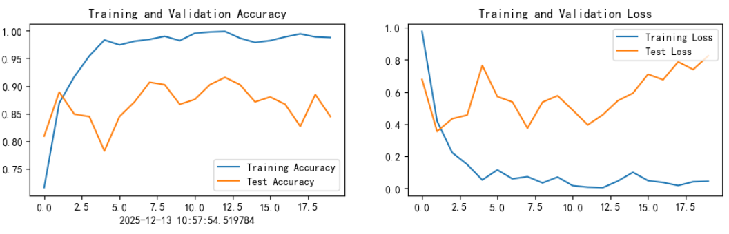

2. 模型评估

best_model.eval()
epoch_test_acc, epoch_test_loss = test(test_dl, best_model, loss_fn)

epoch_test_acc, epoch_test_loss
# 查看是否与我们记录的最高准确率一致
epoch_test_acc

0.9155555555555556

五、YOLOv5-C3模块

YOLO（You Only Look Once）系列模型自 2015 年由 Joseph Redmon 提出 YOLOv1 开始，便以其单阶段（one-stage）实时目标检测架构闻名，将检测任务转化为回归问题，通过一次前向传播同时预测边界框和类别概率。这种设计不同于双阶段模型（如 Faster R-CNN），强调速度和简洁性，但早期版本（如 YOLOv1 到 YOLOv3）在处理小物体或拥挤场景时存在局限，主要依赖 Darknet 框架和残差连接来深化网络。

转折点出现在 2020 年，随着 YOLOv4 的发布（由 Alexey Bochkovskiy 等开发），引入了 CSPNet（Cross Stage Partial Network）架构。这是一种创新的网络设计，旨在解决深层网络中的梯度流动问题和计算冗余。CSPNet 通过将特征图分成两部分——一部分直接传递，另一部分经过密集处理后合并——实现了更好的梯度传播和参数效率。YOLOv4 的主干网络 CSPDarknet-53 正是基于此，显著提升了模型在准确性和速度上的平衡。

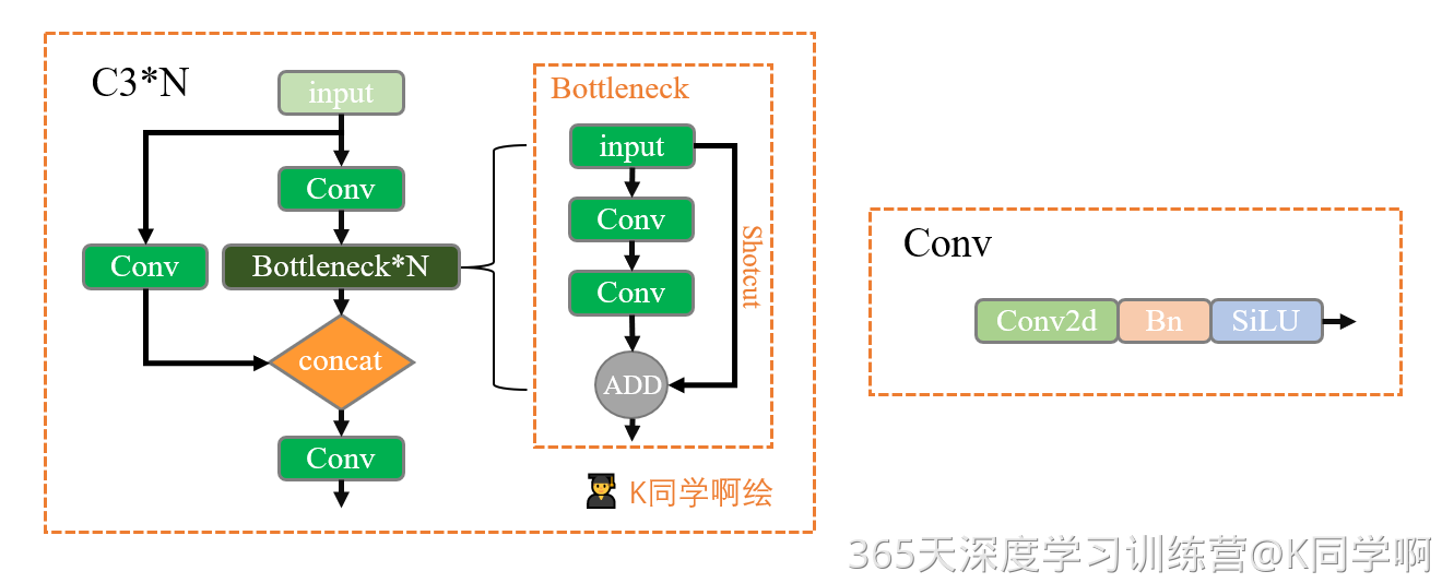
同年，Ultralytics 团队发布了 YOLOv5，这是 YOLO 系列的重大里程碑。它首次完全转向 PyTorch 框架（而非之前的 Darknet），提高了模型的模块化和可移植性，便于训练和部署。YOLOv5 继承了 YOLOv4 的 CSP 思想，但进行了优化：在主干和颈部（neck）引入了 C3 模块（全称 Cross Stage Partial Bottleneck with 3 convolutions）。C3 的构建灵感直接来源于 CSPNet，但专为 YOLOv5 的高效实时检测需求量身定制。它于 2020 年随 YOLOv5 首次亮相，并成为模型的核心构建块，帮助 YOLOv5 在 COCO 数据集上实现更高的 mAP（mean Average Precision）和更低的计算开销。YOLOv5 还推出了多个变体（如 YOLOv5s、m、l、x），通过复合缩放（compound scaling，借鉴 EfficientDet）调整深度和宽度，以适应不同硬件。

C3 模块的开发目的是在保持轻量级的同时，提升特征提取效率。它由三个卷积层组成：输入特征图被分成两支，一支直接通过一个 1x1 卷积进行维度调整，另一支经过瓶颈结构（Bottleneck，通常包括两个 3x3 卷积和残差连接），然后两支合并。这种“跨阶段部分”设计减少了参数量，同时改善了梯度流动，避免深层网络中的信息丢失。在 YOLOv5 的主干中，C3 与 CBS（Conv + BatchNorm + SiLU）模块堆叠，形成高效的特征提取管道；颈部则结合 SPPF（Spatial Pyramid Pooling Fast）模块，进一步处理多尺度特征。