扩散模型从原理到实践-第四周

stevensmj

已于 2023-11-08 15:36:00 修改

阅读量1.8k

点赞数 6

文章标签：算法人工智能

于 2023-11-08 15:33:43 首次发布

本文链接：https://blog.csdn.net/stevensmh/article/details/134286520

版权

任务四：

视频讲解：DDIM反转的应用
DDIM反转
音频扩散模型
打卡内容：
1. 学习笔记
2. 作业：使用DDIM反转技术把demo图片中的小猫替换为小狗

扩散模型的精细控制和拓展应用

DDIM Inversion

DDIM Inversion技术，是基于ODE过程可以在小步长的限制下进行反转的假设。它的采样过程跟DDIM正常采样过程相反，是从 $z_{0}\rightarrow z_{T}$ ，数学表示为：

$z_{t+1}=\sqrt{\alpha_{t+1}}(\frac{z_{t}-\sqrt{1-\alpha_{t}} \cdot \varepsilon(z_{t})}{\sqrt{\alpha_{t}}})+\sqrt{1-\alpha_{t+1}}\cdot \varepsilon(z_{t})$

其中 $z_{0}$ 是给定的真实图像的编码，Inversion最后得到包含原图像信息的噪声编码 $z_T$ ，后面DDIM采样过程以 $z_T$ 为初始值，能够近似重建原图像编码 $z_{0}$ ，因此DDIM Inversion常用于真实图像编辑。

在实践中，DDIM Inversion每一步都会产生误差，对于无条件扩散模型，累积误差可以忽略。但是对基于classifier-free guidance（ w >1 ）的扩散模型，累积误差会不断增加，DDIM Inversion最终获得的噪声向量可能会偏离高斯分布，再经过DDIM采样，最终生成的图像会严重偏离原图像，并可能产生视觉伪影。因此，如果希望 DDIM Inversion之后的采样结果在layout上与原始图像相似，通常使用当引导系数 w = 1, 即无 negative prompt时，DDIM Inversion产生的轨迹提供了原始图像的粗略近似。

DDIM Sampling

下面，通过加载一个名为"runwayml/stable-diffusion-v1-5"的stable diffusion管线，实现这一想法：

import torch
import requests
import torch.nn as nn
import torch.nn.functional as F
from PIL import Image
from io import BytesIO
from tqdm.auto import tqdm
from matplotlib import pyplot as plt
from torchvision import transforms as tfms
from diffusers import StableDiffusionPipeline, DDIMScheduler

device = torch.device("mps" if torch.backends.mps.is_available() else "cuda" if torch.cuda.is_available()

# Useful function for later
def load_image(url, size=None):
    response = requests.get(url,timeout=0.2)
    img = Image.open(BytesIO(response.content)).convert('RGB')
    if size is not None:
        img = img.resize(size)
    return img

# Load a pipeline
pipe = StableDiffusionPipeline.from_pretrained("runwayml/stable-diffusion-v1-5").to(device)


# Set up a DDIM scheduler
pipe.scheduler = DDIMScheduler.from_config(pipe.scheduler.config)

简而言之，DDIM采样是指在特定时间点，嘈杂的图像是原始图像与一些噪声的混合，其中噪声是具有单位方差的高斯噪声。在DDPM论文中，这个高斯噪声的参数被称为'alpha'（α），并且它定义了噪声调度器。在Diffusers中，通过计算alpha调度器的值并将其存储在scheduler.alphas_cumprod中来处理这些值。

# Plot 'alpha' (alpha_bar in DDPM language, alphas_cumprod in Diffusers for clarity)
timesteps = pipe.scheduler.timesteps.cpu()
alphas = pipe.scheduler.alphas_cumprod[timesteps]
plt.plot(timesteps, alphas, label='alpha_t');
plt.legend();

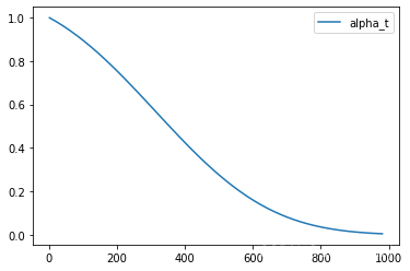
最初（时间步0，图表的左侧），我们从一个干净的图像开始，没有噪音。随着时间步的增加，我们最终几乎全部都是噪音，并且噪音逐渐减少至接近0。

在采样过程中，我们从时间步1000开始，纯粹是噪音，然后慢慢移动到时间步0。为了计算采样轨迹中的下一个时间步（因为我们是从高时间步向低时间步移动），我们预测噪音（这是我们模型的输出），然后使用它来计算预测的去噪图像。然后我们使用这个预测来沿着指向某个方向的小距离移动。最后，我们可以添加一些额外的噪音，按照某个因子缩放。

因此，基于DDIM 的采样过程可以描述为以下代码：

# Sample function (regular DDIM)
@torch.no_grad()
def sample(prompt, start_step=0, start_latents=None,
           guidance_scale=3.5, num_inference_steps=30,
           num_images_per_prompt=1, do_classifier_free_guidance=True,
           negative_prompt='', device=device):
  
    # Encode prompt
    text_embeddings = pipe._encode_prompt(
            prompt, device, num_images_per_prompt, do_classifier_free_guidance, negative_prompt
    )

    # Set num inference steps
    pipe.scheduler.set_timesteps(num_inference_steps, device=device)

    # Create a random starting point if we don't have one already
    if start_latents is None:
        start_latents = torch.randn(1, 4, 64, 64, device=device)
        start_latents *= pipe.scheduler.init_noise_sigma

    latents = start_latents.clone()

    for i in tqdm(range(start_step, num_inference_steps)):
    
        t = pipe.scheduler.timesteps[i]

        # Expand the latents if we are doing classifier free guidance
        latent_model_input = torch.cat([latents] * 2) if do_classifier_free_guidance else latents
        latent_model_input = pipe.scheduler.scale_model_input(latent_model_input, t)

        # Predict the noise residual
        noise_pred = pipe.unet(latent_model_input, t, encoder_hidden_states=text_embeddings).sample

        # Perform guidance
        if do_classifier_free_guidance:
            noise_pred_uncond, noise_pred_text = noise_pred.chunk(2)
            noise_pred = noise_pred_uncond + guidance_scale * (noise_pred_text - noise_pred_uncond)


        # Normally we'd rely on the scheduler to handle the update step:
        # latents = pipe.scheduler.step(noise_pred, t, latents).prev_sample

        # Instead, let's do it ourselves:
        prev_t = max(1, t.item() - (1000//num_inference_steps)) # t-1
        alpha_t = pipe.scheduler.alphas_cumprod[t.item()]
        alpha_t_prev = pipe.scheduler.alphas_cumprod[prev_t]
        predicted_x0 = (latents - (1-alpha_t).sqrt()*noise_pred) / alpha_t.sqrt()
        direction_pointing_to_xt = (1-alpha_t_prev).sqrt()*noise_pred
        latents = alpha_t_prev.sqrt()*predicted_x0 + direction_pointing_to_xt

    # Post-processing
    images = pipe.decode_latents(latents)
    images = pipe.numpy_to_pil(images)

    return images

我们测试一个例子如下：

# Test our sampling function by generating an image
sample('Watercolor painting of a beach sunset', negative_prompt=negative_prompt, num_inference_st

Inversion Concept

下面我们将用具体的代码来显示 DDIM Inversion 这个概念。

# https://www.pexels.com/photo/a-beagle-on-green-grass-field-8306128/
input_image = load_image('https://images.pexels.com/photos/8306128/pexels-photo-8306128.jpeg', size=(512, 512))
input_image


input_image_prompt = "Photograph of a puppy on the grass"

# Encode with VAE
with torch.no_grad(): latent = pipe.vae.encode(tfms.functional.to_tensor(input_image).unsqueeze(0).to(device)*2-1)
l = 0.18215 * latent.latent_dist.sample()

## Inversion
@torch.no_grad()
def invert(start_latents, prompt, guidance_scale=3.5, num_inference_steps=80,
           num_images_per_prompt=1, do_classifier_free_guidance=True,
           negative_prompt='', device=device):
  
    # Encode prompt
    text_embeddings = pipe._encode_prompt(
            prompt, device, num_images_per_prompt, do_classifier_free_guidance, negative_prompt
    )

    # Latents are now the specified start latents
    latents = start_latents.clone()

    # We'll keep a list of the inverted latents as the process goes on
    intermediate_latents = []

    # Set num inference steps
    pipe.scheduler.set_timesteps(num_inference_steps, device=device)

    # Reversed timesteps <<<<<<<<<<<<<<<<<<<<
    timesteps = reversed(pipe.scheduler.timesteps)

    for i in tqdm(range(1, num_inference_steps), total=num_inference_steps-1):

        # We'll skip the final iteration
        if i >= num_inference_steps - 1: continue

        t = timesteps[i]

        # Expand the latents if we are doing classifier free guidance
        latent_model_input = torch.cat([latents] * 2) if do_classifier_free_guidance else latents
        latent_model_input = pipe.scheduler.scale_model_input(latent_model_input, t)

        # Predict the noise residual
        noise_pred = pipe.unet(latent_model_input, t, encoder_hidden_states=text_embeddings).sample

        # Perform guidance
        if do_classifier_free_guidance:
            noise_pred_uncond, noise_pred_text = noise_pred.chunk(2)
            noise_pred = noise_pred_uncond + guidance_scale * (noise_pred_text - noise_pred_uncond)

        current_t = max(0, t.item() - (1000//num_inference_steps)) #t
        next_t = t # min(999, t.item() + (1000//num_inference_steps)) # t+1
        alpha_t = pipe.scheduler.alphas_cumprod[current_t]
        alpha_t_next = pipe.scheduler.alphas_cumprod[next_t]

        # Inverted update step (re-arranging the update step to get x(t) (new latents) as a function of x(t-1) (current latents)
        latents = (latents - (1-alpha_t).sqrt()*noise_pred)*(alpha_t_next.sqrt()/alpha_t.sqrt()) + (1-alpha_t_next).sqrt()*noise_pred


        # Store
        intermediate_latents.append(latents)
            
    return torch.cat(intermediate_latents)

这个函数与上面的采样函数相似，但我们在时间步上沿着相反的方向移动，从t=0开始，向更高噪音的方向移动。不同之处在于，我们不是更新我们的潜在变量以减少噪音，而是估计预测的噪音并使用它来撤销一个更新步骤，将它们从t移动到t+1。

下面使用这个 invert 函数来创建一系列中间表示：

inverted_latents = invert(l, input_image_prompt, num_inference_steps=50)
inverted_latents.shape

# Decode the final inverted latents
with torch.no_grad():
  im = pipe.decode_latents(inverted_latents[-1].unsqueeze(0))
pipe.numpy_to_pil(im)[0]

上面是其中最后一层中间表示的可视化图像，也是加噪声最多的一张图，此时已经很难分辨出原始的小狗图片，但是接下来，我们将基于这个噪声图片，作为新的采样起始点，生成一系列不同的新图片（基于一些新的prompt）。在新的图片里面，与原始图像相匹配，但在与新提示相关的地方有所不同。

# Sampling with a new prompt
start_step = 10
new_prompt = input_image_prompt.replace('puppy', 'cat')
sample(new_prompt, start_latents=inverted_latents[-(start_step+1)][None], 
       start_step=start_step, num_inference_steps=50)[0]

通过 new prompt 能够将原始图片中的 puppy 替换为 cat，并且周围的环境是相似的，可以看作好像我们直接对图像进行了 edit 导致原图中的 puppy这一概念被替换为了 cat 概念，并且其他的地方都没有发生大的变动。

现在我们将创建一个整合的 edit 函数，从而将上面所有的分步操作结合在一起：

from PIL import Image
import numpy as np

def edit_image_with_inversion(input_image, input_image_prompt, edit_prompt, num_steps=100, start_step=30, guidance_scale=3.5):
    with torch.no_grad(): latent = pipe.vae.encode(tfms.functional.to_tensor(input_image).unsqueeze(0).to(device)*2-1)
    l = 0.18215 * latent.latent_dist.sample()
    inverted_latents = invert(l, input_image_prompt, num_inference_steps=num_steps)
    final_im = sample(edit_prompt, start_latents=inverted_latents[-(start_step+1)][None], 
                      start_step=start_step, num_inference_steps=num_steps, guidance_scale=g

    return final_im

尝试更多的 new prompt:

edit(input_image, 'A puppy on the grass', 'an old grey dog on the grass', num_steps=50, start_step=10)

edit(input_image, 'A puppy on the grass', 'A blue dog on the lawn', num_steps=50, start_step=12,

更多的步骤 = 更好的性能，如果您在使用较不精确的反演时遇到问题，您可以尝试使用更多的步骤（代价是更长的运行时间）。为了测试反演，您可以使用我们的编辑函数，并使用相同的提示：

# Inversion test with far more steps
edit(input_image, 'A puppy on the grass', 'A puppy on the grass', num_steps=350, start_step=1)

edit(input_image, 'A photograph of a puppy', 'A photograph of a grey cat', num_steps=150, start_

Null-text Inversion

问题：DDIM inversion 在有 guidance 的情形下并不能较好地重建输入，该如何找到更好的inversion方式？

如上图上半部分所示，设 DDIM inversion 过程为 $z^*_0\rightarrow z^*_1\rightarrow z^*_2\rightarrow ...\rightarrow z^*_T$ ，往回采样的过程为 $z^*_T\rightarrow \overline{z}_{T-1}\rightarrow ...\rightarrow \overline{z}_{1}\rightarrow \overline{z}_{0}$ . 二者每一步都会有一定的误差，在没有 guidance（即 w =1 ）的情形下，这些误差比较小，重建结果还是能几乎还原图像的。但是当 w >1 时，这些误差会被放大，导致重建结果与原图有明显的差异。而实践中我们常常依靠大 guidance scale（如 w =7.5 ）来生成高质量图像，因此这个问题必须得到解决。

我们现在仔细考虑采样过程的每一步。如上图下半部分所示，classifier-free guidance 会让网络推理两次，分别对应有条件（上分支）和无条件（下分支），二者结果依据 w 做线性组合得到这一步的最终预测值。由于 prompt-to-prompt 方法要利用文本条件和 attention map 之间的关系，所以我们并不想改变条件分支和网络权重，于是我们能改变的只有无条件分支的输入，也即 null-text embedding $\phi_t$ . 我们希望通过优化 $\phi_t$ ，使得采样过程能够重建出原图，这就是该方法的名字 null-text inversion 的意义。考虑到 w =1 下的 DDIM inversion 能较好的重建原图，我们自然想到以 $z^*_{T-1}$ 作为目标，让 $\overline{z}_{T-1}$ 去接近它，因此损失函数就是二者的 MSE.

$min\left \| z^*_{T-1} - \overline{z}_{T-1}\right \|^2_2$

按照扩散过程 t=T→1 的顺序对每个时间步 t 的采样执行单独的优化，尽可能使inversion proess接近samping process，那么新轨迹将在 z0 附近结束，从而保留原图像的语义和视觉信息。

实现上，由于采样过程是随时间步进行的，因此我们要按 t=T→1 的顺序逐步训练——当前一步训练好之后，在前一步的采样基础之上训练下一步。另外，虽然原本的 null-text 对应的 embedding 只有一个全局的 ∅ ，但是作者发现为每一步都定义自己的 $\phi_t$ 能大幅提高性能。综上所述，训练算法如下图所示：

总结一下，Null-text inversion 的亮点在于它揭示了 classifier-free guidance 下，结果受无条件分支的影响非常大，并成功地利用这种影响达到了重建输入图像的目的.

Diffusion for Audio

From Audio to Image and Back Again

使用 diffusion 模型来制作 audio 的本质上，其实是通过diffusion模型生成对应的 spectrogram 图像，再在此频谱图上做进一步的后处理得到对应的 audio。

下面是一个简单的 spectrogram 与 audio 直接的互相转换。这里使用 mel spectrogram，以帮助人耳能够识别的有效信息得以凸显出来。

import torch, random
import numpy as np
import torch.nn.functional as F
from tqdm.auto import tqdm
from IPython.display import Audio
from matplotlib import pyplot as plt
from diffusers import DiffusionPipeline
from torchaudio import transforms as AT
from torchvision import transforms as IT


# Load a pre-trained audio diffusion pipeline
device = "mps" if torch.backends.mps.is_available() else "cuda" if torch.cuda.is_available() else "cpu"
pipe = DiffusionPipeline.from_pretrained("teticio/audio-diffusion-instrumental-hiphop-256").to(device)


# Sample from the pipeline and display the outputs
output = pipe()
display(output.images[0])
display(Audio(output.audios[0], rate=pipe.mel.get_sample_rate()))

pipe.mel

Mel {
  "_class_name": "Mel",
  "_diffusers_version": "0.12.0.dev0",
  "hop_length": 512,
  "n_fft": 2048,
  "n_iter": 32,
  "sample_rate": 22050,
  "top_db": 80,
  "x_res": 256,
  "y_res": 256
}

通过使用函数image_to_audio() 来实现从频谱图到音频的转换，使用函数 audio_slice_to_image() 可以实现从音乐片段到对应频谱图的转换。

a = pipe.mel.image_to_audio(output.images[0])
a.shape

pipe.mel.load_audio(raw_audio=a)
im = pipe.mel.audio_slice_to_image(0)
im

sample_rate_pipeline = pipe.mel.get_sample_rate()
sample_rate_pipeline

Fine-Tuning the pipeline

首先加载来自 'lewtun/music_genres' 的数据集：

from datasets import load_dataset
dataset = load_dataset('lewtun/music_genres', split='train')
dataset

audio_array = dataset[0]['audio']['array']
sample_rate_dataset = dataset[0]['audio']['sampling_rate']
print('Audio array shape:', audio_array.shape)
print('Sample rate:', sample_rate_dataset)
display(Audio(audio_array, rate=sample_rate_dataset))

a = dataset[0]['audio']['array'] # Get the audio array
pipe.mel.load_audio(raw_audio=a) # Load it with pipe.mel
pipe.mel.audio_slice_to_image(0) # View the first 'slice' as a spectrogram

sample_rate_dataset = dataset[0]['audio']['sampling_rate']
sample_rate_dataset

Audio array shape: (1323119,)
Sample rate: 44100

44100

请注意，这个音频的采样率较高 - 如果我们想要使用现有的流程，我们需要对其进行“重新采样”以匹配。音频片段的长度也比流程设置的要长。幸运的是，当我们使用pipe.mel加载音频时，它会自动将音频剪切成较小的部分。在这里，我们使用torchaudio的转换（作为AT导入）来进行重新采样，使用pipe的mel将音频转化为图像，然后使用torchvision的转换（作为IT导入）将图像转化为张量。这样，我们就得到了一个将音频片段转化为可用于训练的频谱图张量的函数：

resampler = AT.Resample(sample_rate_dataset, sample_rate_pipeline, dtype=torch.float32)
to_t = IT.ToTensor()

def to_image(audio_array):
  audio_tensor = torch.tensor(audio_array).to(torch.float32)
  audio_tensor = resampler(audio_tensor)
  pipe.mel.load_audio(raw_audio=np.array(audio_tensor))
  num_slices = pipe.mel.get_number_of_slices()
  slice_idx = random.randint(0, num_slices-1) # Pic a random slice each time (excluding the last short slice)
  im = pipe.mel.audio_slice_to_image(slice_idx) 
  return im

我们将使用我们的to_image()函数作为自定义collate函数的一部分，将我们的数据集转化为一个数据加载器（dataloader），以便用于训练。collate函数定义了如何将数据集中的一批示例转化为最终用于训练的批处理数据。在这种情况下，我们将每个音频样本转化为频谱图像，然后将生成的张量堆叠在一起：

def collate_fn(examples):
  # to image -> to tensor -> rescale to (-1, 1) -> stack into batch
  audio_ims = [to_t(to_image(x['audio']['array']))*2-1 for x in examples]
  return torch.stack(audio_ims)

# Create a dataset with only the 'Chiptune / Glitch' genre of songs
batch_size = 4 # 4 on colab, 12 on A100
chosen_genre = 'Electronic' # <<< Try training on different genres <<<
indexes = [i for i, g in enumerate(dataset['genre']) if g == chosen_genre]
filtered_dataset = dataset.select(indexes)
dl = torch.utils.data.DataLoader(filtered_dataset.shuffle(), batch_size=batch_size, collate_fn=collate_fn, shuffle=True)
batch = next(iter(dl))
print(batch.shape)

最后，我们定义一个训练过程如下：

epochs = 3
lr = 1e-4

pipe.unet.train()
pipe.scheduler.set_timesteps(1000)
optimizer = torch.optim.AdamW(pipe.unet.parameters(), lr=lr)

for epoch in range(epochs):
    for step, batch in tqdm(enumerate(dl), total=len(dl)):
        
        # Prepare the input images
        clean_images = batch.to(device)
        bs = clean_images.shape[0]

        # Sample a random timestep for each image
        timesteps = torch.randint(
            0, pipe.scheduler.num_train_timesteps, (bs,), device=clean_images.device
        ).long()

        # Add noise to the clean images according to the noise magnitude at each timestep
        noise = torch.randn(clean_images.shape).to(clean_images.device)
        noisy_images = pipe.scheduler.add_noise(clean_images, noise, timesteps)

        # Get the model prediction
        noise_pred = pipe.unet(noisy_images, timesteps, return_dict=False)[0]

        # Calculate the loss
        loss = F.mse_loss(noise_pred, noise)
        loss.backward(loss)

        # Update the model parameters with the optimizer
        optimizer.step()
        optimizer.zero_grad()



output = pipe()
display(output.images[0])
display(Audio(output.audios[0], rate=22050))

最终我们可以得到基于 “Electronic” 电子音乐 style 的歌曲和对应的spectrogram：

此外，我们还可以通过输入更大的起始 noise image 来得到更长的 audio 片段。

# Make a longer sample by passing in a starting noise tensor with a different shape
noise = torch.randn(1, 1, pipe.unet.sample_size[0], pipe.unet.sample_size[1]*4).to(device)
output = pipe(noise=noise)
display(output.images[0])
display(Audio(output.audios[0], rate=22050))

stevensmj

关注

6
点赞
踩
9

收藏

觉得还不错? 一键收藏
1
评论
扩散模型从原理到实践-第四周

DDIM Inversion每一步都会产生误差，对于无条件扩散模型，累积误差可以忽略。但是对基于classifier-free guidance（w >1）的扩散模型，累积误差会不断增加，DDIM Inversion最终获得的噪声向量可能会偏离高斯分布，再经过DDIM采样，最终生成的图像会严重偏离原图像，并可能产生视觉伪影。
复制链接

扫一扫