TensorFlow实现卷积神经网络（进阶）

此模型中如果使用100k个batch，并结合学习速率的decay（即每隔一段时间将学习速率下降一个比率），正确率可以高达86%。模型中需要训练的参数约为100万个，而预测时需要进行的四则运算总量在2000万次左右。所以这个卷积神经网络模型中，使用一些技巧。
（1）对weight进行L2的正则化。
（2）对图片进行翻转，随机剪切等数据增强，制造更多样本。
（3）在每个卷积-最大池化层后面使用LRN层，增强模型的泛化能力。

---

卷积加池化的组合目前已经是做图像识别的一个标准组件了。卷积层主要做特征提取，全连接层开始多特征进行组合匹配，并进行分类。卷积层的训练相对于全连接层更复杂，训练全连接层基本是进行一些矩阵的乘法运算。

---

下载TensorFow Model，在构建模型时会用到读取CTFAR-10数据的类（cifar10.py和cifar10_input.py）（CTFAR-10一个经典的数据集）

git clone git@github.com:tensorflow/models.git
cd models/tutorials/image/cifar10 

卷积神经网络结构：
conv1 卷积层和激活函数
pool1 最大池化
norm1 LRN
conv2 卷积层和激活函数
norm2 LRN
pool2 最大池化层
local3 全连接层和激活函数
local4 全连接层和激活函数
logits 模型Inference的输出结果

# coding:UTF-8
# 载入常用库，NumPy的time，并载入TlensorFow Models中的自动下载、读取CIFAR-10数据的类。
import cifar10,cifar10_input
import tensorflow as tf
import numpy as np
import time

########输入数据########
# 训练论数、batch大小（3000个batch，每个batch包含128个样本）。
max_steps = 3000
batch_size = 128
# 下载CIFAR-10数据的默认路径
data_dir = '/tmp/cifar10_data/cifar-10-batches-bin'

########初始化权重########
# 定义初始化weight的函数，依然使用tf.truncated_normal截断的正态分布来初始化权重。
# 这里给weight加一个L2的loss，相当于做了一个L2的正则化处理。这个collection名为“losses”，会在后面计算总体loss时被用上
def variable_with_weight_loss(shape, stddev, wl):
    var = tf.Variable(tf.truncated_normal(shape, stddev = stddev))
    if wl is not None:
        weight_loss = tf.multiply(tf.nn.l2_loss(var), wl, name = 'weight_loss')
        tf.add_to_collection('losses', weight_loss)
    return var

########数据处理########
# 把cifar10的数据解压到data_dir中，然后将下一行代码注释掉，取消运行
# (用到cifar-10.py)使用CIFAR-10下载数据集，并解压展开到其默认位置
cifar10.maybe_download_and_extract()

# 使用cifar10_input类中的distorted_input函数产生训练需要使用的数据，返回的是已经封装好的tensor，每次执行都会生成一个batch_size的数量的样本。
images_train, labels_train = cifar10_input.distorted_inputs(data_dir = data_dir, batch_size = batch_size)

# 使用cifar10_input.inputs函数生成测试数据。需要裁剪图片正中间的24*24的区块，并进行数据标准化操作。
images_test, labels_test = cifar10_input.inputs(eval_data = True, data_dir = data_dir, batch_size = batch_size)

# 创建输入数据的placeholder。batche_size在之后定义网络结构时被用到了，所以数据尺寸的第一个值样本条数需要提前设定。
image_holder = tf.placeholder(tf.float32, [batch_size, 24, 24, 3])
label_holder = tf.placeholder(tf.int32, [batch_size])

########设计网络结构########
# 第一个卷积层
# 创建卷积核并进行初始化，不对第一个卷积层的weight进行L2正则
weight1 = variable_with_weight_loss(shape = [5,5,3,64], stddev = 5e-2, wl = 0.0)
# 对输入数据进行卷积操作
kernel1 = tf.nn.conv2d(image_holder, weight1, [1,1,1,1], padding = 'SAME')
# 这层的bias全部初始化为0，再将卷积的结果加上bias
bias1 = tf.Variable(tf.constant(0.0, shape = [64]))
# 使用激活函数进行非线性化
conv1 = tf.nn.relu(tf.nn.bias_add(kernel1, bias1))
# 使用尺寸为3*3且步长为2*2的最大池化层处理数据，最大池化层的尺寸和步长不一致，增加数据的丰富性
pool1 = tf.nn.max_pool(conv1, ksize = [1,3,3,1], strides = [1,2,2,1], padding = 'SAME')
# 使用LRN对结果进行处理，对局部神经元的活动创建竞争环境，增强模型的泛化能力
norm1 = tf.nn.lrn(pool1, 4, bias = 1.0, alpha = 0.001/9.0, beta = 0.75)

# 第二个卷积层（与上一层相似）
# 上一层的卷积核数量为64（即输出64个通道）。本层卷积核的第三维度输入通道数为64。
weight2 = variable_with_weight_loss(shape = [5,5,64,64], stddev = 5e-2, wl = 0.0)
kernel2 = tf.nn.conv2d(norm1, weight2, [1,1,1,1], padding = 'SAME')
# bias值全部初始化为0.1。
bias2 = tf.Variable(tf.constant(0.1, shape = [64]))
conv2 = tf.nn.relu(tf.nn.bias_add(kernel2, bias2))
# 与上一层不同，先进行LRN处理，在进行最大池化层。
norm2 = tf.nn.lrn(conv2, 4, bias = 1.0, alpha = 0.001/9.0, beta = 0.75)
pool2 = tf.nn.max_pool(norm2, ksize = [1,3,3,1], strides = [1,2,2,1], padding = 'SAME')

# 全连接层
# 将上一层的输出结果进行flatten。tf.reshape函数将每个样本都变成一维向量。
reshape = tf.reshape(pool2, [batch_size, -1])
# 获取数据扁平化之后的长度。
dim = reshape.get_shape()[1].value
# 对全连接层的weight进行初始化，隐含节点数为384，正太分布的标准差0.04。设置非零的weight loss，这一程所有参数被L2正则约束。
weight3 = variable_with_weight_loss(shape = [dim, 384], stddev = 0.04, wl = 0.004)
# bias值初始化为0.1
bias3 = tf.Variable(tf.constant(0.1, shape = [384]))
# 使用激活函数进行非线性化
local3 = tf.nn.relu(tf.matmul(reshape, weight3) + bias3)

# 全连接层（与上一层类似）
# 隐含层节点数下降一半只有192个，其他超参数保持不变
weight4 = variable_with_weight_loss(shape = [384,192], stddev = 0.04, wl = 0.004)
bias4 = tf.Variable(tf.constant(0.1, shape = [192]))
local4 = tf.nn.relu(tf.matmul(local3, weight4) + bias4)

# 输出层（把Softmax的操作放在了loss部分）
# 创建weight，其正态分布标准差为上一层隐含节点的倒数，并且不计入L2的正则。
weight5 = variable_with_weight_loss(shape = [192,10], stddev = 1/192.0, wl = 0.0)
bias5 = tf.Variable(tf.constant(0.0, shape = [10]))
# Softmax放在下面的原因。我们不需要对inference的输出进行softmax处理就可以获得最终的分类结果。 
# 直接比较inference输出的各类的数值大小即可。计算softmax主要是为了计算loss。因此softmax操作整合到后面合适。
# 模型Inference的输出结果
logits = tf.nn.relu(tf.matmul(local4, weight5) + bias5)

########计算CNN的loss########
# softmax和cross entropy loss的计算合在一起
# 得到最终的loss，其中包括cross entropy loss和后两个全连接层weight的L2 loss
def loss(logits, labels):
    labels = tf.cast(labels, tf.int64)
    cross_entropy = tf.nn.sparse_softmax_cross_entropy_with_logits(logits = logits, labels = labels, name = 'cross_entropy_per_example')
    cross_entropy_mean = tf.reduce_mean(cross_entropy, name = 'cross_entropy')
    tf.add_to_collection('losses', cross_entropy_mean)
    return tf.add_n(tf.get_collection('losses'), name = 'total_loss')
# loss函数中传入值，获得最终的loss
loss = loss(logits, label_holder)


########训练设置 ########
# 选择优化器，学习速率设为1e-3
train_op = tf.train.AdamOptimizer(1e-3).minimize(loss)
# 输出结果中top k的准确率，也就是输出分数最高的那一类的准确率
top_k_op = tf.nn.in_top_k(logits, label_holder, 1)

# 创建默认的Session
sess = tf.InteractiveSession()
# 初始化全部模型参数
tf.global_variables_initializer().run()
# 启动图片数据增强的线程队列，一共使用16个线程进行加速。不启动无法开始后面的inference
tf.train.start_queue_runners()

########开始训练########
# 记录每个step花费的时间，每隔10个step计算并展示当前的loss、每秒能训练的样本数量，以及在一个batch花费的时间。
for step in range(max_steps):
    start_time = time.time()
    # 在每一个step的训练过程，先获得一个batch数据。再将这个batch数据传入train_op和loss的计算。
    image_batch, label_batch = sess.run([images_train, labels_train])
    _, loss_value = sess.run([train_op, loss], 
            feed_dict = {image_holder: image_batch, label_holder: label_batch})
    duration = time.time() - start_time
    if step %10 ==0:
        examples_per_sec = batch_size / duration
    sec_per_batch = float(duration)
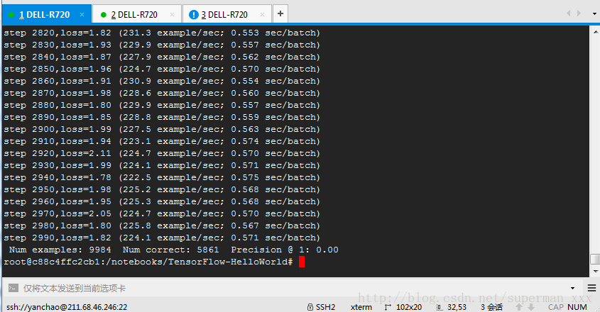
        format_str = ('step %d,loss=%.2f (%.1f example/sec; %.3f sec/batch)')
    print(format_str % (step, loss_value, examples_per_sec, sec_per_batch))

# 测试集评测准确率
# 测试集样本数
num_examples = 10000
import math
# 计算多少个batch能将全部样本评测完
num_iter = int(math.ceil(num_examples / batch_size))
true_count = 0
total_sample_count = num_iter * batch_size
step = 0
# 在每一个的step中使用Session的run方法获取test的batch
# 再执行top_k_op计算模型在这个batch的top 1上预测正确的样本数。
# 最后汇总所有预测正确的结果，求得全部测试样本中预测正确的数量。
while step < num_iter:
    image_batch, label_batch = sess.run([images_test,labels_test])
    predictions = sess.run([top_k_op], feed_dict = {image_holder: image_batch, label_holder: label_batch})
    true_count += np.sum(predictions)
    step += 1
# 最后将准确率评测结果计算并打印出来。
precision = true_count / total_sample_count
# print('precision @ 1 = %.3f' % precision)

print (' Num examples: %d  Num correct: %d  Precision @ 1: %0.02f ' % (
total_sample_count, true_count, precision))