sklearn 决策树

决策树

简介

• 决策树与SVM一样，都是非常通用的机器学习算法，可以用于分类或者回归问题，以及多输出问题
• 决策树是之后的集成方法：随机森林的一个基础模块，RF是将生成很多决策树，并进行模型预测
• 决策树对于数据预处理的要求较低，它的节点主要是条件语句，因此不需要对数据对标准化或者归一化操作。
• 对于决策树的结果，其特征的重要性程度是可以解释的，是white box模型。而像RF和NN这些算法，都是黑盒模型

训练和可视化

• 直接利用sklearn中的DecisionTreeClassifier就可以实现基于决策树的分类，如果要对分类结果进行可视化，则需要用到graphviz软件

判别

• 采用gini纯度来对节点的分类能力进行判断
  $${G_i} = 1 - \sum\limits_{k = 1}^n {p_{i,k}^2}$$
  $p_{i,k}$是标签k的第i个节点中，属于类别k的训练样本数
• sklearn中使用CART算法进行决策树的分类，每个不是叶子的节点都有2个子节点

估计类的概率

• 决策树会估计样本属于类别的概率，最大概率所在的类别就是样本的类别

CART(Classifcation And Regression Tree)算法

• CART算法的原理：挑选出一个特征$k$和一个阈值$t_k$，将这个子集下的所有样本分为两类，对于特定的节点，在每次的分类过程中，代价函数(我们需要最小化的函数)为
  $$J(k,{t_k}) = \frac{{{m_{left}}}}{m}{G_{left}} + \frac{{{m_{right}}}}{m}{G_{right}}$$
  $G_{left/right}$是左右子集的Gini系数，用于检测子节点的纯度，$m_{left/right}$是左右子集的样本个数
• 算法使用相同的逻辑将子集进行分类，直到树到达最大的深度或者找不到一个可以降低纯度的分割方法，还有一些其他的超参数用于停止算法的迭代，如下
  
  • min_samples_split：子节点小于这个数，就不会再进行分割
  • min_samples_leaf：叶子的样本个数小于这个数，就不会进行此次分割
  • min_weight_fraction_leaf：分割后，叶子的样本比例小于这个数，就不会进行此次分割
  • max_leaf_nodes：最大的叶子节点个数
• CART算法是贪婪算法，它在每一步只搜索当前的最优解，不能保证最终得到的是全局最优解
• 平均来说，CART算法的时间复杂度为:$O(n \cdot m \cdot log(m))$
• 除了Gini纯度作为代价函数，也可以设置熵纯度( entropy impurity)，熵越小，表示系统静止或有序，表示一个能量较低的状态
  某个节点的熵为
  $${H_i} = - \sum\limits_{k = 1,{p_{i,k}} \ne 0}^n {{p_{i,k}}\log ({p_{i,k}})}$$
• 大部分情况下，Gini纯度与熵纯度得到的树都类似，Gini纯度的计算速度比熵纯度要稍微快一点；相对于Gini纯度，熵纯度作为代价函数得到的树会更加平衡

正则化超参数

• 决策树不对训练数据做出什么假设，即比如说数据符合线性模型等，因此常常会对训练数据过拟合。这样的模型也可以成为非参数模型。因为参数个数是由训练数据确定的。而对于参数化模型来说，其参数个数是预确定的，模型的自由度有限，因此也就降低了过拟合的风险。
• 为了降低决策树过拟合的危险，可以引入上面提到的一些参数

import os
import numpy as np
from sklearn.datasets import load_iris
from sklearn.tree import DecisionTreeClassifier
from sklearn.tree import export_graphviz
iris = load_iris()
X = iris.data[:,2:]
y = iris.target

tree_clf = DecisionTreeClassifier( max_depth=2 )
tree_clf.fit( X, y )

# 导出图
# export_graphviz( tree_clf,
#                  out_file="images/decision_trees/tree_clf.dot",
#                  feature_names=iris.feature_names[2:],
#                  class_names=iris.target_names,
#                 rounded=True,
#                 filled=True
#                 )
print( tree_clf.predict_proba([[5, 1.5]]) )
print(tree_clf.predict([[5, 1.5]]))

[[ 0.          0.33333333  0.66666667]]
[2]

%matplotlib inline
import matplotlib.pyplot as plt
from matplotlib.colors import ListedColormap

def plot_decision_boundary(clf, X, y, axes=[0, 7.5, 0, 3], iris=True, legend=False, plot_training=True):
    x1s = np.linspace(axes[0], axes[1], 100)
    x2s = np.linspace(axes[2], axes[3], 100)
    x1, x2 = np.meshgrid(x1s, x2s)
    X_new = np.c_[x1.ravel(), x2.ravel()]
    y_pred = clf.predict(X_new).reshape(x1.shape)
    custom_cmap = ListedColormap(['#fafab0','#9898ff','#a0faa0'])
    plt.contourf(x1, x2, y_pred, alpha=0.3, cmap=custom_cmap, linewidth=10)
    if not iris:
        custom_cmap2 = ListedColormap(['#7d7d58','#4c4c7f','#507d50'])
        plt.contour(x1, x2, y_pred, cmap=custom_cmap2, alpha=0.8)
    if plot_training:
        plt.plot(X[:, 0][y==0], X[:, 1][y==0], "yo", label="Iris-Setosa")
        plt.plot(X[:, 0][y==1], X[:, 1][y==1], "bs", label="Iris-Versicolor")
        plt.plot(X[:, 0][y==2], X[:, 1][y==2], "g^", label="Iris-Virginica")
        plt.axis(axes)
    if iris:
        plt.xlabel("Petal length", fontsize=14)
        plt.ylabel("Petal width", fontsize=14)
    else:
        plt.xlabel(r"$x_1$", fontsize=18)
        plt.ylabel(r"$x_2$", fontsize=18, rotation=0)
    if legend:
        plt.legend(loc="lower right", fontsize=14)
    return

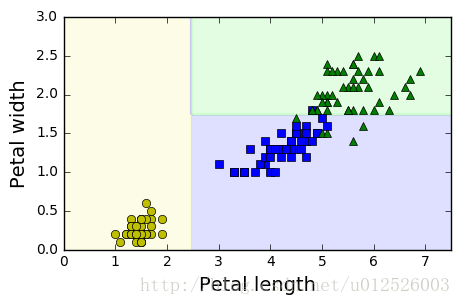
plt.figure(figsize=(5, 3))
plot_decision_boundary(tree_clf, X, y)
plt.show()

# 添加的这个超参数可以有效地降低模型的过拟合程度
from sklearn.datasets import make_moons
Xm, ym = make_moons(n_samples=100, noise=0.25, random_state=53)

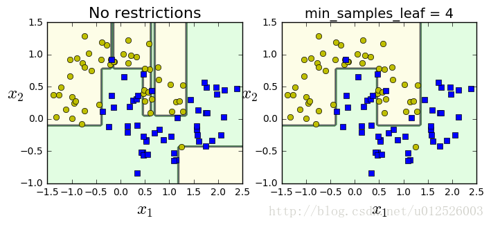
deep_tree_clf1 = DecisionTreeClassifier(random_state=42)
deep_tree_clf2 = DecisionTreeClassifier(min_samples_leaf=4, random_state=42)
deep_tree_clf1.fit(Xm, ym)
deep_tree_clf2.fit(Xm, ym)

plt.figure(figsize=(8, 3))
plt.subplot(121)
plot_decision_boundary(deep_tree_clf1, Xm, ym, axes=[-1.5, 2.5, -1, 1.5], iris=False)
plt.title("No restrictions", fontsize=16)
plt.subplot(122)
plot_decision_boundary(deep_tree_clf2, Xm, ym, axes=[-1.5, 2.5, -1, 1.5], iris=False)
plt.title("min_samples_leaf = {}".format(deep_tree_clf2.min_samples_leaf), fontsize=14)

plt.show()

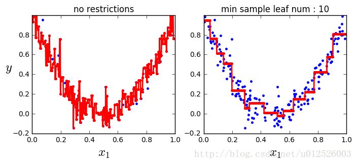
回归问题

• 与分类问题类似，对于回归问题，首先需要构建一棵树，需要求某个样本的值的时候，首先找到该样本所在的叶子节点，然后对该节点上的所有值取平均，就是该样本的平均值，每个节点都有对应的mse
• 回归问题的代价函数是
  $$\begin{array}{l} J(k,{t_k}) = \frac{{{m_{left}}}}{m}MS{E_{left}} + \frac{{{m_{right}}}}{m}MS{E_{right}}\\ where & \left\{ \begin{array}{l} MS{E_{node}} = \sum\limits_{i \in node} {{{({{\hat y}_{node}} - {y^{(i)}})}^2}} \\ {{\hat y}_{node}} = \frac{1}{{{m_{node}}}}\sum\limits_{i \in node} {{y^{(i)}}} \end{array} \right. \end{array}$$
• 如果没有一些正则化参数，决策树回归模型也很容易发生过拟合

from sklearn.tree import DecisionTreeRegressor

np.random.seed(42)
m = 200
X = np.random.rand(m, 1)
y = 4 * (X - 0.5) ** 2
y = y + np.random.randn(m, 1) / 10

from sklearn.tree import DecisionTreeRegressor

tree_reg = DecisionTreeRegressor(max_depth=2, random_state=42)
tree_reg.fit(X, y)

tree_reg1 = DecisionTreeRegressor(random_state=42)
tree_reg2 = DecisionTreeRegressor(random_state=42, min_samples_leaf=10)
tree_reg1.fit(X, y)
tree_reg2.fit(X, y)

def plot_regression_predictions(tree_reg, X, y, axes=[0, 1, -0.2, 1], ylabel="$y$"):
    x1 = np.linspace(axes[0], axes[1], 500).reshape(-1, 1)
    y_pred = tree_reg.predict(x1)
    plt.axis(axes)
    plt.xlabel("$x_1$", fontsize=18)
    if ylabel:
        plt.ylabel(ylabel, fontsize=18, rotation=0)
    plt.plot(X, y, "b.")
    plt.plot(x1, y_pred, "r.-", linewidth=2, label=r"$\hat{y}$")

plt.figure(figsize=(8, 3))
plt.subplot(121)
plot_regression_predictions(tree_reg1, X, y)
plt.title("no restrictions")
plt.subplot(122)
plot_regression_predictions(tree_reg2, X, y, ylabel=None)
plt.title("min sample leaf num : 10")
plt.show()

一些缺点

• 不稳定：决策树的决策边界关于特征的方向是正交的，因此模型对于训练集的旋转十分敏感，可以采用PCA对数据进行预处理，避免训练集的方向对模型结果的影响
• 决策树对训练集数据十分敏感，训练集稍微修改一下，决策树形状都可能发生很大的变化