强化学习（2） Actor-Critic演员评论家（ A2C, Cliff Walking PlayGround）Pytorch实例

原文

Pytorch实现Actor Critic Baseline (A2C, Cliff Walking PlayGround) | 文艺数学君这一篇简单介绍使用Pytorch在环境Cliff Walking PlayGround上实现Actor-Critic Baseline (A2C). 因为目前很少有使用Cliff Walking作为A2C的例子, 这里就做一个简单的说明. 最后会把原始的notebook文件上传Github.https://mathpretty.com/12665.html

略加修改

 一、Actor-Critic算法简介

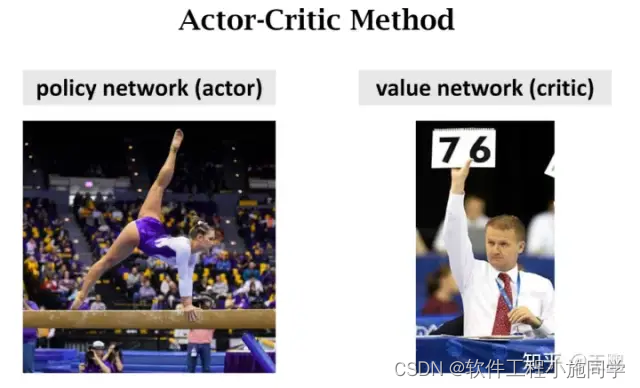
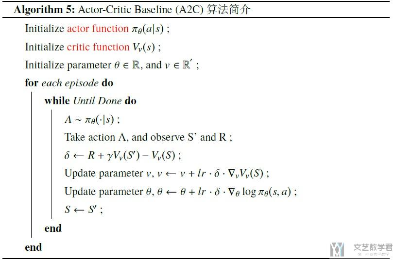
Actor-Critic从名字上看包括两部分，演员(Actor)和评价家(Critic)。

Actor使用的是策略函数，输入状态S，负责选择动作(Action)。

Critic使用的是价值函数，输入状态S，负责评估Actor的表现，并指导Actor下一阶段的动作。

这一篇介绍在Policy Gradient中的Actor Critic Baseline, 也就是常说的A2C. 这一篇的实验环境还是使用Cliff Walking PlayGround, 使用Google Colab完成实验.

Google Colab免费GPU使用教程-CSDN博客文章浏览阅读4.9k次，点赞9次，收藏77次。有时候本地跑代码可能耗时比较久，而且还会耽误你本地电脑的使用，购买云服务器又不舍得买，所以我们可以使用谷歌的免费服务器，可以使用GPU跑代码Google Colab官网是一个免费的基于云端的Jupyter笔记本环境，由Google提供。它提供了一个方便的平台，使用户可以创建、分享和协作编写Python代码和机器学习模型。以下是是免费的，无需购买任何硬件或软件。使用Google的云端计算机，使用户能够在云端上运行代码，而不必担心自己的电脑性能和存储空间。Jupyter基于Jupyter。_google colabhttps://blog.csdn.net/niulinbiao/article/details/133953684

这一篇会简单介绍一下Policy Gradient with Baseline的算法过程 (关于具体的推导, 放在之后来讲), 本文会使用Pytorch实现简单的A2C.

1.参考资料

• 关于本实验的代码, 见Github仓库, 07_Actor_Critic_Baseline_(A2C)_Pytorch.ipynb
• 本实验参考的代码, Pytorch-Actor-Critic.py
• 关于环境的介绍, Reinforcement Learning(强化学习)-Cliff Walking Playground环境介绍
• 关于Pytorch实现DQN的代码, Pytorch实现Deep Q-Learning(Cliff Walking PlayGround)
• 封面图片来源, Reinforcement Learning: How Tech Teaches Itself

2. Actor Critic Baseline的介绍

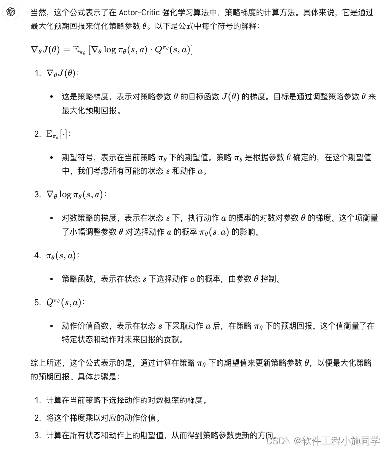
Actor Critic是Policy Gradient算法. 它的想法就是希望可以找到一个函数, 来近似Policy, 给这个函数state, 返回的是每一个动作的action. 一般我们会称这个policy为Pi.

为了更新这个策略, 我们需要定义目标函数, 目标函数是希望累计reward尽可能大. 经过化简有以下的形式, 其中Pi(s,a)是用来根据state, 给出action的概率. 除此之外, 我们还需要估计state-action value, 也就是Q值.

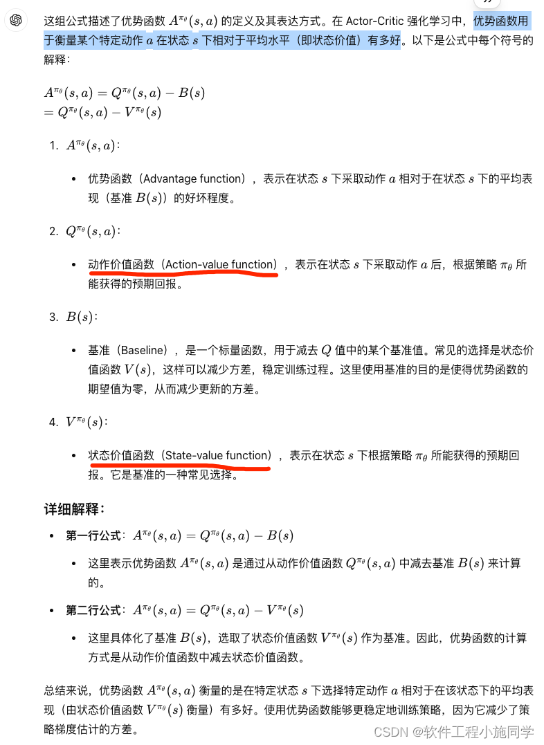
为了减少方差, 我们定义了一个advantage function, 为A = Q - V, 目的是保持上面的期望不变, 方差减少. 如下所示, 但是这样有一个问题, 就是我们需要近似三个函数, 分别是Pi, Q, V.

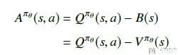
但是, 我们可以证明V的TD误差是上面A的无偏估计. 所以最终的梯度公式可以化简为如下的形式.

其中:

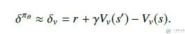
其中Pi和V我们都可以使用神经网络进行代替, 梯度也是可以进行求的. 于是上面的式子就是可以求得.

3. Actor Critic Baseline算法流程

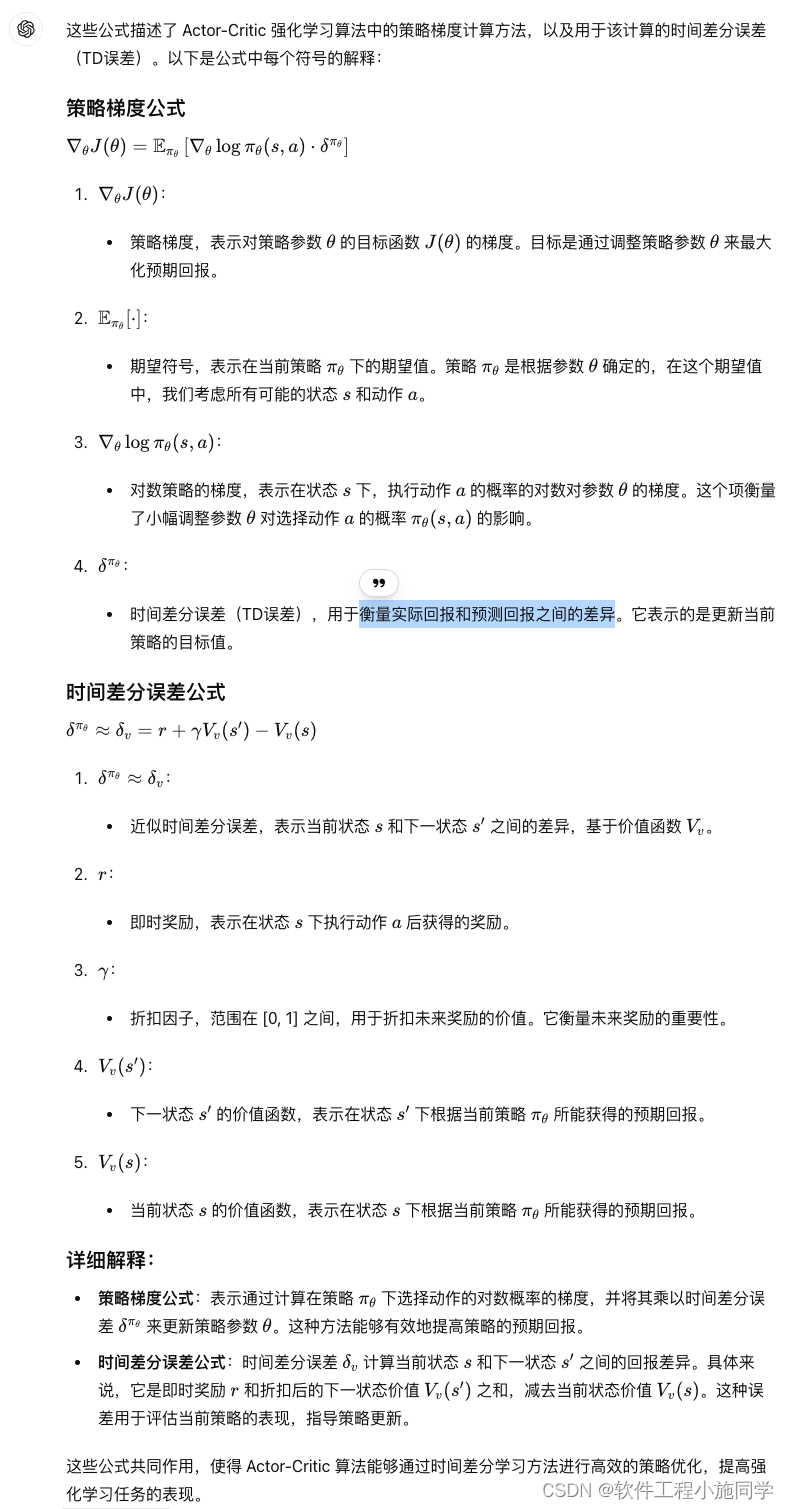
我们把上面的方法稍作归纳, 可以写成下面的形式.

其中:

• 为了更新critic function, 我们设置loss function为(V-Gt)^2, 求导后与上面的式子相同.
• 为了更新actor function, 我们设置loss function为-log_prob * (Gt - V), 这里我们增加负号, 于是可以使用梯度下降来进行参数更新.

下面是我从Actor critic algorithm看到的, 很好的介绍了算法的流程, 就放在这里做一个总体的参考.

二、Pytorch实现Actor Critic Baseline (A2C)

这里我们只给出关键部分的代码, 完整的notebook可以查看github仓库,

1.初始化环境

我们这里还是使用Cliff Walking Playground, 在该环境中智能体在一个 4x12 的网格中移动，状态编号如下所示：

[[ 0,  1,  2,  3,  4,  5,  6,  7,  8,  9, 10, 11], [12, 13, 14, 15, 16, 17, 18, 19, 20, 21, 22, 23], [24, 25, 26, 27, 28, 29, 30, 31, 32, 33, 34, 35], [36, 37, 38, 39, 40, 41, 42, 43, 44, 45, 46, 47]]

在任何阶段开始时，初始状态都是状态 36，状态 47 是唯一的终止状态，悬崖对应的是状态 37 到 46。智能体有 4 个可选动作（UP = 0，RIGHT = 1，DOWN = 2，LEFT = 3）。

智能体每走一步都会得到-1 的奖励，跌入悬崖会得到-100 的奖励并重置到起点，当达到目标时，片段结束。

先初始化环境.

1. env = CliffWalkingEnv()

接着我们定义一个函数, 来获取当前的state. 因为在Cliff Walking Playground只会返回当前的state, 也就是一个数字, 我们在这里将其转换为one-hot的向量（只有一个元素为1，其余所有元素都为0）

def get_screen(state):
    """这里我们就用state来作为例子, 不直接使用截图了, 将编号转换为one-hot向量, 共48维
    """

    # 创建特定类型的张量，比如[[1]]
    y_state = torch.Tensor([[state]]).long()
    # 创建了一个形状为 (1, 48) 的二维张量。这意味着张量有 1 行和 48 列
    y_onehot = torch.FloatTensor(1, 48) # 产生位置

    # In your for loop
    y_onehot.zero_() # 全部使用0进行填充
    # 第 1 行的第 3 列的值设置为 1
    y_onehot.scatter_(1, y_state, 1) # 返回one-hot
    return y_onehot

比如说, 如果环境返回的是state=1, 那么该函数就可以生成如下的向量.

get_screen(1)
"""
tensor([[0., 1., 0., 0., 0., 0., 0., 0., 0., 0., 0., 0., 0., 0., 0., 0., 0., 0.,
         0., 0., 0., 0., 0., 0., 0., 0., 0., 0., 0., 0., 0., 0., 0., 0., 0., 0.,
         0., 0., 0., 0., 0., 0., 0., 0., 0., 0., 0., 0.]])
"""

2.定义Actor Critic的模型

首先我们简单来看一下Actor和Critic这两个模型的输入和输出.

• Actor模型的输入是state, 输出是每一个action的概率.
• Critic模型的输入是state, 输入是这个state对应的value.

所以这两个模型的输入部分都是对state的处理, 所以我们可以将这两个网络的前几层进行共享.

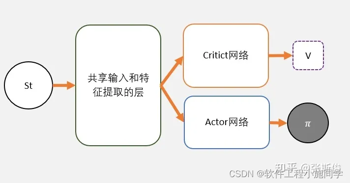
下面我们定义模型, 定义在一个class里面, 输出部分由两个部分组成.

import torch.nn as nn  # 导入PyTorch的神经网络模块
import torch.nn.functional as F  # 导入PyTorch的神经网络函数模块

# 定义一个ActorCriticModel类，继承自nn.Module
class ActorCriticModel(nn.Module):
    def __init__(self):
        super(ActorCriticModel, self).__init__()  # 调用父类nn.Module的构造函数
        self.fc1 = nn.Linear(48, 24)  # 定义第一个全连接层，输入维度为48，输出维度为24
        self.fc2 = nn.Linear(24, 12)  # 定义第二个全连接层，输入维度为24，输出维度为12
        self.action = nn.Linear(12, 4)  # 定义第三个全连接层，输入维度为12，输出维度为4，用于输出动作概率
        self.value = nn.Linear(12, 1)  # 定义第四个全连接层，输入维度为12，输出维度为1，用于输出状态值

    # x是状态
    def forward(self, x):
        x = F.relu(self.fc1(x))  # 将输入x传入第一个全连接层并通过ReLU激活函数
        x = F.relu(self.fc2(x))  # 将经过第一个全连接层的输出传入第二个全连接层并通过ReLU激活函数
        # dim=-1表示‘按’最后一个维度进行softmax，对于二维，那么最后一维就是列，那么就是softmaxt每行
        action_probs = F.softmax(self.action(x), dim=-1)  # 将第二个全连接层的输出传入第三个全连接层并通过softmax函数计算动作概率
        state_values = self.value(x)  # 将第二个全连接层的输出传入第四个全连接层计算状态值
        return action_probs, state_values  # 返回动作概率和状态值

这段代码定义了一个Actor-Critic模型，其中：

• fc1 和 fc2 是用于特征提取的全连接层。
• action 层输出动作的概率分布。
• value 层输出状态值。
• forward 方法定义了前向传播的过程，输入数据经过两个全连接层和ReLU激活函数后，分成两路：一路通过softmax函数输出动作概率，另一路输出状态值。

于是, Actor模型和Critic模型的结构分别如下:

• Actor模型的结构是, 48->24->12->4;
• Critic模型的结构是, 48->24->12->1;

前面两层的参数是共享的. 这个网络的输出有两个, 一个是actor模型的返回, 每个action的概率, 另一个是这个state的value值. 我们简单看一下这个网络的返回.

ac = ActorCriticModel()
# tensor.squeeze(dim) 方法用于去除指定维度上的大小为 1 的维度
# x 是一个形状为 [1, 48] 的二维张量。squeeze(0) 将去除第一个维度，因为它的大小为 1。这样，结果将是一个形状为 [48] 的一维张量
action_probs, state_values = ac(get_screen(1).squeeze(0))
print(action_probs)
print(state_values)
"""
tensor([0.2140, 0.3271, 0.2130, 0.2459], grad_fn=<SoftmaxBackward>)
tensor([-0.3331], grad_fn=<AddBackward0>)
"""

3.模型的训练

在这里我们使用MC的方式来进行训练.

"MC" 通常指的是 Monte Carlo 方法，用于估计状态值或动作值，通过从环境中生成随机样本路径（即从开始状态到终止状态的序列）并计算这些路径的回报来进行学习。

我们会完成一个完整的episode, 这个时候可以获得如下的一组数据:

• 当前state的累计收益(Gt, 这个是实际计算的);
• 对当前state收益的估计(V值);
• 当前state采取一个action的概率的log值, 即对应下面代码中的log_probs;

接着, 我们可以计算actor loss和critic loss. 这两个loss的计算分别如下:

• critic loss = (V-Gt)^2, 也就是希望我们对状态state的价值估计与其实际价值相似.
• actor loss = -log_prob * (Gt - V), 我们称作Gt-V为advantage function.

于是, 将上面的想法合起来, 就组成了下面的代码.

def trainIters(env, ActorCriticModel, num_episodes, gamma=0.9):
    """
    使用Actor-Critic方法训练强化学习模型。

    参数:
    env: gym.Env
        强化学习环境，用于交互和获取状态、奖励等信息。
    
    ActorCriticModel: torch.nn.Module
        训练的Actor-Critic模型，用于计算动作概率和状态值。
    
    num_episodes: int
        训练的episode数量，每个episode代表一次完整的环境交互直到终止状态。
    
    gamma: float, 可选，默认值为0.9
        折扣因子，用于计算未来奖励的折扣值。较小的gamma值使模型更注重短期奖励，较大的gamma值使模型更注重长期奖励。
    """
    # 使用Adam优化器，学习率为0.03
    optimizer = torch.optim.Adam(ActorCriticModel.parameters(), 0.03)
    # 设置学习率调度器，每10步将学习率缩放0.9倍
    scheduler = torch.optim.lr_scheduler.StepLR(optimizer, step_size=10, gamma=0.9)
    # 记录每个episode的累计奖励和进行的长度
    stats = plotting.EpisodeStats(
        episode_lengths=np.zeros(num_episodes+1),
        episode_rewards=np.zeros(num_episodes+1))
    
    # 训练多个episode
    for i_episode in range(1, num_episodes+1):
        # 重置环境，获取初始状态
        state = env.reset()
        # 将状态转换为one-hot张量，用作网络输入
        state = get_screen(state)
        
        # 初始化存储log概率、奖励和状态值的列表
        log_probs = []
        rewards = []
        state_values = []
        
        # 进行每个时间步的训练
        for t in itertools.count():
            # 获取当前状态下不同动作的概率和状态值
            action_probs, state_value = ActorCriticModel(state.squeeze(0))
            # 依据动作概率选择一个动作
            # 从当前状态下的动作概率分布中随机选择一个动作，并返回该动作的索引
            # 根据给定的概率分布进行采样，选择动作的概率与每个动作的概率值成正比
            action = torch.multinomial(action_probs, 1).item()
            # 记录选择动作的log概率
            log_prob = torch.log(action_probs[action])
            # 执行动作，获得下一个状态、奖励和是否结束标志
            next_state, reward, done, _ = env.step(action)
            
            # 更新统计数据
            stats.episode_rewards[i_episode] += reward
            stats.episode_lengths[i_episode] = t
            
            # 将奖励转换为张量
            reward = torch.tensor([reward], device=device)
            # 将下一个状态转换为张量
            next_state_tensor = get_screen(next_state)
            
            # 将log概率、奖励和状态值存入列表
            # view(-1)将log_prob张量转换成一维张量
            log_probs.append(log_prob.view(-1))
            rewards.append(reward)
            state_values.append(state_value)
            
            # 更新当前状态
            state = next_state_tensor
            
            # 如果一轮结束，开始更新网络参数
            if done:
                returns = []
                Gt = 0    # 累计收益
                pw = 0    # 当前时间步距离序列终点的偏移量（power），用于计算未来奖励的折扣系数。
                
                # 计算每个时间步的回报
                for reward in rewards[::-1]:
                    # 在计算未来回报（discounted reward）时，需要考虑每个奖励距离当前时间步的远近，越远的奖励其折扣系数越大
                    Gt = Gt + (gamma ** pw) * reward
                    pw += 1
                    returns.append(Gt)
                
                # 将回报列表反转，使其对应时间步
                returns = returns[::-1]
                # 将回报转换为张量并标准化
                # .cat()将一系列张量沿指定维度进行连接
                returns = torch.cat(returns)
                returns = (returns - returns.mean()) / (returns.std() + 1e-9)
                
                # 将log概率和状态值转换为张量
                log_probs = torch.cat(log_probs)
                state_values = torch.cat(state_values)
                
                # 计算优势函数
                # detach(): 从计算图中分离出张量，创建一个新的张量，该张量不再参与反向传播
                advantage = returns.detach() - state_values
                # 计算critic的损失
                critic_loss = F.smooth_l1_loss(state_values, returns.detach())
                # 计算actor的损失
                actor_loss = (-log_probs * advantage.detach()).mean()
                # 总损失为critic损失和actor损失之和
                loss = critic_loss + actor_loss
                
                # 更新网络参数
                optimizer.zero_grad()
                loss.backward()
                optimizer.step()
                
                # 打印当前episode的信息
                print('Episode: {}, total steps: {}'.format(i_episode, t))
                
                # 如果时间步超过20步，调整学习率
                if t > 20:
                    scheduler.step()
                
                # 跳出时间步循环，进入下一个episode
                break
    
    # 返回训练统计数据
    return stats

上面代码可以说是由两个部分组成的:

• 对于每一个episode, 我们都进行模型, 使用actor生成动作, 并使用critic得到对state的评价, 将其分别存入数组中.
• 当一个episode结束后, 我们根据返回的reward, 分别计算每一个state的累计reward. 也就是上面for reward in reward[::-1]部分的代码. 接着就是计算两个的loss, 并进行反向传播, 更新网络参数.

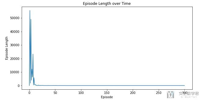
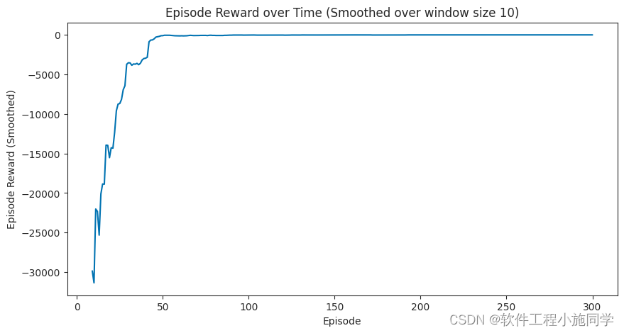
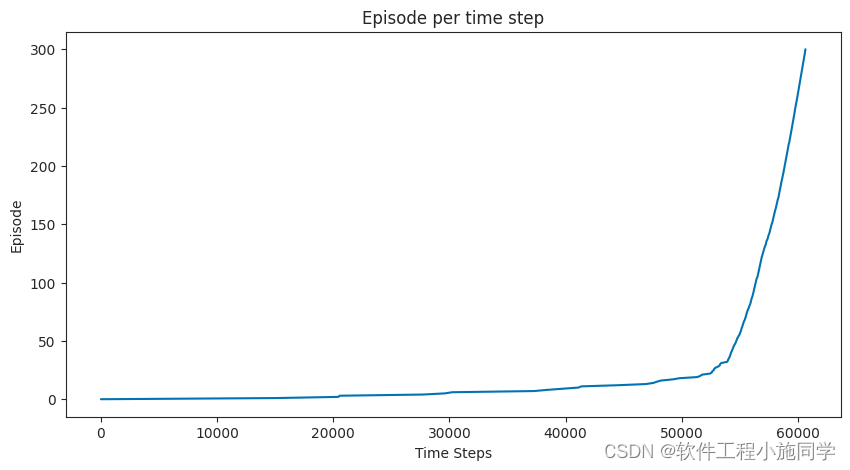
大概可以在20个episode之后模型收敛.

4.一些注意点

上面的代码中, 有几个小的tricks, 在这里说明一下. 第一个是一定要对returns进行归一化处理. 也就是下面这句语句.

1. returns = (returns - returns.mean()) / (returns.std() + 1e-9)

如果去掉之后, 好像是不能收敛的.

第二个是关于计算Gt的时候, 如果已经是tensor的格式, 不能使用简写符号, 这样会使得内存共享, 导致最后returns数组里的结果是完全一些的. 也就是不能写成下面的形式>

1. Gt += (gamma ** pw) * reward,

需要写成下面的形式, 这一这里说的情况是reward已经是tensor的格式了.

1. Gt = Gt + (gamma ** pw) * reward

5. 完整代码

1. plotting.py

reinforcement-learning/lib/plotting.py at master · dennybritz/reinforcement-learning · GitHubImplementation of Reinforcement Learning Algorithms. Python, OpenAI Gym, Tensorflow. Exercises and Solutions to accompany Sutton's Book and David Silver's course. - reinforcement-learning/lib/plotting.py at master · dennybritz/reinforcement-learninghttps://github.com/dennybritz/reinforcement-learning/blob/master/lib/plotting.py

import matplotlib
import numpy as np
import pandas as pd
from collections import namedtuple
from matplotlib import pyplot as plt
from mpl_toolkits.mplot3d import Axes3D

EpisodeStats = namedtuple("Stats",["episode_lengths", "episode_rewards"])

def plot_cost_to_go_mountain_car(env, estimator, num_tiles=20):
    x = np.linspace(env.observation_space.low[0], env.observation_space.high[0], num=num_tiles)
    y = np.linspace(env.observation_space.low[1], env.observation_space.high[1], num=num_tiles)
    X, Y = np.meshgrid(x, y)
    Z = np.apply_along_axis(lambda _: -np.max(estimator.predict(_)), 2, np.dstack([X, Y]))

    fig = plt.figure(figsize=(10, 5))
    ax = fig.add_subplot(111, projection='3d')
    surf = ax.plot_surface(X, Y, Z, rstride=1, cstride=1,
                           cmap=matplotlib.cm.coolwarm, vmin=-1.0, vmax=1.0)
    ax.set_xlabel('Position')
    ax.set_ylabel('Velocity')
    ax.set_zlabel('Value')
    ax.set_title("Mountain \"Cost To Go\" Function")
    fig.colorbar(surf)
    plt.show()


def plot_value_function(V, title="Value Function"):
    """
    Plots the value function as a surface plot.
    """
    min_x = min(k[0] for k in V.keys())
    max_x = max(k[0] for k in V.keys())
    min_y = min(k[1] for k in V.keys())
    max_y = max(k[1] for k in V.keys())

    x_range = np.arange(min_x, max_x + 1)
    y_range = np.arange(min_y, max_y + 1)
    X, Y = np.meshgrid(x_range, y_range)

    # Find value for all (x, y) coordinates
    Z_noace = np.apply_along_axis(lambda _: V[(_[0], _[1], False)], 2, np.dstack([X, Y]))
    Z_ace = np.apply_along_axis(lambda _: V[(_[0], _[1], True)], 2, np.dstack([X, Y]))

    def plot_surface(X, Y, Z, title):
        fig = plt.figure(figsize=(20, 10))
        ax = fig.add_subplot(111, projection='3d')
        surf = ax.plot_surface(X, Y, Z, rstride=1, cstride=1,
                               cmap=matplotlib.cm.coolwarm, vmin=-1.0, vmax=1.0)
        ax.set_xlabel('Player Sum')
        ax.set_ylabel('Dealer Showing')
        ax.set_zlabel('Value')
        ax.set_title(title)
        ax.view_init(ax.elev, -120)
        fig.colorbar(surf)
        plt.show()

    plot_surface(X, Y, Z_noace, "{} (No Usable Ace)".format(title))
    plot_surface(X, Y, Z_ace, "{} (Usable Ace)".format(title))



def plot_episode_stats(stats, smoothing_window=10, noshow=False):
    # Plot the episode length over time
    fig1 = plt.figure(figsize=(10,5))
    plt.plot(stats.episode_lengths)
    plt.xlabel("Episode")
    plt.ylabel("Episode Length")
    plt.title("Episode Length over Time")
    if noshow:
        plt.close(fig1)
    else:
        plt.show(fig1)

    # Plot the episode reward over time
    fig2 = plt.figure(figsize=(10,5))
    rewards_smoothed = pd.Series(stats.episode_rewards).rolling(smoothing_window, min_periods=smoothing_window).mean()
    plt.plot(rewards_smoothed)
    plt.xlabel("Episode")
    plt.ylabel("Episode Reward (Smoothed)")
    plt.title("Episode Reward over Time (Smoothed over window size {})".format(smoothing_window))
    if noshow:
        plt.close(fig2)
    else:
        plt.show(fig2)

    # Plot time steps and episode number
    fig3 = plt.figure(figsize=(10,5))
    plt.plot(np.cumsum(stats.episode_lengths), np.arange(len(stats.episode_lengths)))
    plt.xlabel("Time Steps")
    plt.ylabel("Episode")
    plt.title("Episode per time step")
    if noshow:
        plt.close(fig3)
    else:
        plt.show(fig3)

    return fig1, fig2, fig3

 2. main.py

# -*- coding: utf-8 -*-
"""“Actor-Critic  Baseline (A2C) Pytorch.ipynb”的副本

Automatically generated by Colab.

Original file is located at
    https://colab.research.google.com/drive/1jDV4FBVfaRxZjFRsJToMqBPjBzcn73xq
"""

from google.colab import drive
drive.mount('/content/drive')

import sys
if "/content/drive/My Drive/Machine Learning/lib/" not in sys.path:
    sys.path.append("/content/drive/My Drive/Machine Learning/lib/")

# Commented out IPython magic to ensure Python compatibility.

from gym.envs.toy_text import CliffWalkingEnv
import plotting

import gym
import math
import numpy as np
import random
import itertools
from collections import namedtuple, defaultdict

import torch
import torch.nn as nn
import torch.optim as optim
import torch.nn.functional as F

import matplotlib.pyplot as plt
# %matplotlib inline

device = torch.device('cuda' if torch.cuda.is_available() else 'cpu')
device

"""## 测试环境"""

env = CliffWalkingEnv()

def get_screen(state):
    """这里我们就用state来作为例子, 不直接使用截图了, 将编号转换为one-hot向量, 共48维
    """
    y_state = torch.Tensor([[state]]).long()
    y_onehot = torch.FloatTensor(1, 48) # 产生位置
    # In your for loop
    y_onehot.zero_() # 全部使用0进行填充
    y_onehot.scatter_(1, y_state, 1) # 返回one-hot
    return y_onehot

get_screen(1)

"""## 建立模型"""

class ActorCriticModel(nn.Module):
    def __init__(self):
        super(ActorCriticModel, self).__init__()
        self.fc1 = nn.Linear(48, 24)
        self.fc2 = nn.Linear(24, 12)
        self.action = nn.Linear(12, 4)
        self.value = nn.Linear(12, 1)
    def forward(self, x):
        x = F.relu(self.fc1(x))
        x = F.relu(self.fc2(x))
        action_probs = F.softmax(self.action(x), dim=-1)
        state_values = self.value(x)
        return action_probs, state_values

ac = ActorCriticModel()
action_probs, state_values = ac(get_screen(1).squeeze(0))
print(action_probs)
print(state_values)

ac = ActorCriticModel()
action_probs, state_values = ac(get_screen(1))
print(action_probs)
print(state_values)

from torchsummary import summary

summary(ac.to(device), get_screen(1).size())

"""## 开始训练"""


def trainIters(env, ActorCriticModel, num_episodes, gamma = 0.9):
    optimizer = torch.optim.Adam(ActorCriticModel.parameters(), 0.03) # 注意学习率的大小
    scheduler = torch.optim.lr_scheduler.StepLR(optimizer, step_size=10, gamma=0.9)

    # 记录reward和总长度的变化
    stats = plotting.EpisodeStats(
        episode_lengths=np.zeros(num_episodes+1),
        episode_rewards=np.zeros(num_episodes+1))

    for i_episode in range(1, num_episodes+1):
        # 开始一轮游戏
        state = env.reset() # 环境重置
        state = get_screen(state) # 将state转换为one-hot的tensor, 用作网络的输入.

        log_probs = []
        rewards = []
        state_values = []

        for t in itertools.count():
            action_probs, state_value = ActorCriticModel(state.squeeze(0)) # 返回当前state下不同action的概率

            action = torch.multinomial(action_probs, 1).item() # 选取一个action
            log_prob = torch.log(action_probs[action])
            next_state, reward, done, _, _ = env.step(action) # 获得下一个状态

            # 计算统计数据
            stats.episode_rewards[i_episode] += reward # 计算累计奖励
            stats.episode_lengths[i_episode] = t # 查看每一轮的时间

            # 将值转换为tensor
            reward = torch.tensor([reward], device=device)
            next_state_tensor = get_screen(next_state)

            # 将信息存入List
            log_probs.append(log_prob.view(-1))
            rewards.append(reward)
            state_values.append(state_value)

            # 状态更新
            state = next_state_tensor

            if done: # 当一轮结束之后, 开始更新
                returns = []

                Gt = 0
                pw = 0

                # print(rewards)
                for reward in rewards[::-1]:
                    Gt = Gt + (gamma ** pw) * reward # 写成Gt += (gamma ** pw) * reward, 最后returns里东西都是一样的
                    # print(Gt)
                    pw += 1
                    returns.append(Gt)

                returns = returns[::-1]

                returns = torch.cat(returns)
                returns = (returns - returns.mean()) / (returns.std() + 1e-9)
                # print(returns)
                log_probs = torch.cat(log_probs).to(device)
                state_values = torch.cat(state_values).to(device)

                # print(returns)
                # print(log_probs)
                # print(state_values)

                returns = returns.to(device)

                advantage = returns.detach() - state_values

                critic_loss = F.smooth_l1_loss(state_values, returns.detach())
                actor_loss = (-log_probs * advantage.detach()).mean()
                loss = critic_loss + actor_loss

                # 更新critic
                optimizer.zero_grad()
                loss.backward()
                optimizer.step()

                print('Episode: {}, total steps: {}'.format(i_episode, t))

                if t>20:
                    scheduler.step()

                break

    return stats

ActorCritic = ActorCriticModel()
stats = trainIters(env, ActorCritic, 300)


plot_episode_stats(stats)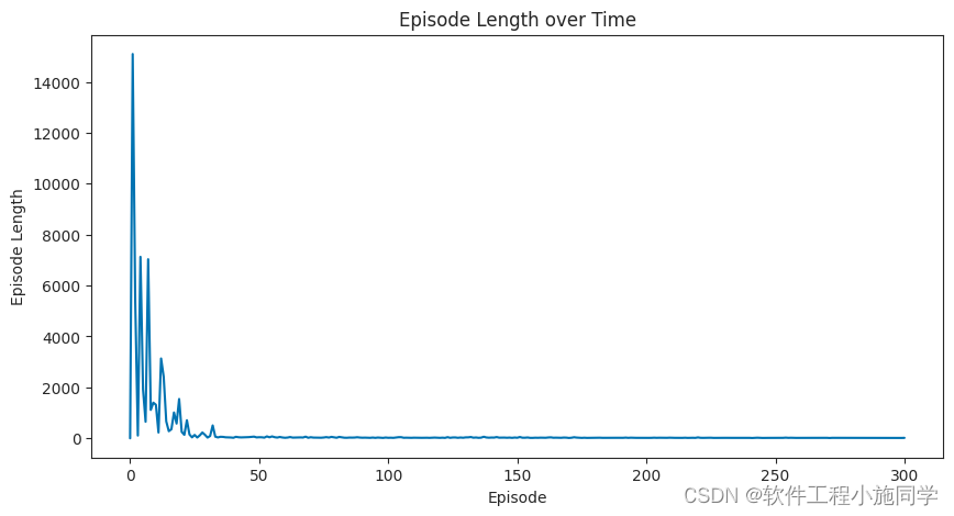

DQN和AC有什么区别，请看

【他山之石】理解Actor-Critic的关键是什么？(附代码及代码分析)关于AC，很多书籍和教程都说AC是DQN和PG的结合。个人觉得道理是怎么个道理，但其实是不够清晰，也很容易产生误读，甚至错误理解AC。至于是在哪里容易产生误读，我会在讲解的时候为你说明。https://mp.weixin.qq.com/s/6zJIZNsPEOM-qwXr2NHDeQ