岭回归+k折交叉验证+正则化调优

import pandas as pd
import numpy as np
from sklearn.model_selection import train_test_split, GridSearchCV
from sklearn.linear_model import Ridge
from sklearn.preprocessing import MinMaxScaler
from sklearn.metrics import mean_squared_error, mean_absolute_error, r2_score
import matplotlib.pyplot as plt
import pickle

# 读取数据
data = pd.read_excel(r'D:\a新模型代码\建模数据.xlsx')

# 数据预处理
X = data[['湿度', 'CO2', '光照', '土壤温度', '土壤湿度']]  # 特征变量
y = data['温度']  # 目标变量

# 特征缩放（标准化）
scaler = MinMaxScaler()
X_scaled = scaler.fit_transform(X)

# 定义岭回归模型
ridge = Ridge()

# 设置正则化参数的候选值
param_grid = {'alpha': np.logspace(-4, 4, 10)}  # 对数尺度上的alpha值

# 使用GridSearchCV进行参数调优，同时进行10折交叉验证
grid_search = GridSearchCV(estimator=ridge, param_grid=param_grid, cv=10, scoring='neg_mean_squared_error')
grid_search.fit(X_scaled, y)

# 获取最优参数
best_alpha = grid_search.best_params_['alpha']
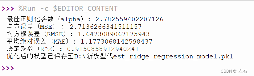
print(f"最佳正则化参数（alpha）: {best_alpha}")

# 使用找到的最佳参数重新训练模型
best_ridge = Ridge(alpha=best_alpha)
best_ridge.fit(X_scaled, y)

# 重新划分训练集和测试集
X_train, X_test, y_train, y_test = train_test_split(X_scaled, y, test_size=0.2, random_state=42)

# 在测试集上进行预测
y_pred = best_ridge.predict(X_test)

# 计算评价指标
mse = mean_squared_error(y_test, y_pred)
rmse = np.sqrt(mse)
mae = mean_absolute_error(y_test, y_pred)
r2 = r2_score(y_test, y_pred)

print("均方误差（MSE）：", mse)
print("均方根误差（RMSE）:", rmse)
print("平均绝对误差（MAE）:", mae)
print("决定系数（R^2）:", r2)

# 绘制结果和保存模型的代码保持不变
# ...（此处省略了与之前相同的绘图和保存模型的代码，因为这部分代码没有改变）
# 可视化预测结果及误差分析
plt.figure(figsize=(10, 6))
plt.rcParams['font.sans-serif'] = ['SimSun']  # 设置中文字体为宋体
plt.rcParams['font.serif'] = ['Times New Roman']  # 设置英文字体为新罗马
# plt.rcParams['font.sans-serif'] = ['SimHei']  # 指定默认字体  
plt.rcParams['axes.unicode_minus'] = False  # 解决保存图像是负号'-'显示为方块的问题
plt.rcParams['font.size'] = 20  # 设置字体大小
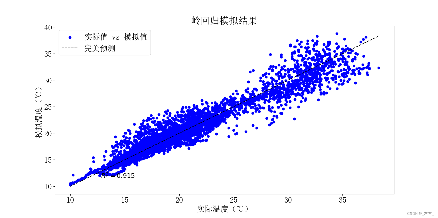
plt.scatter(y_test, y_pred, color='blue', label='实际值 vs 模拟值')
plt.plot([min(y_test), max(y_test)], [min(y_test), max(y_test)], '--k', label='完美预测')
plt.xlabel('实际温度（℃）')
plt.ylabel('模拟温度（℃）')
plt.title('岭回归模拟结果')
plt.legend()
plt.text(
    max(y_test) - (max(y_test) - min(y_test)) * 0.9,
    min(y_test) + (max(y_test) - min(y_test)) * 0.05,
    f'$R^2 = {r2:.3f}$',
    fontsize=16,
    color='black',
    ha='left',
    va='bottom'
)
plt.show()

# 限制只显示前200个样本的对比
subset_size = 200
if len(y_test) > subset_size:
    test_index_subset = np.arange(subset_size)
    y_test_subset = y_test[:subset_size]
    y_pred_subset = y_pred[:subset_size]
else:
    test_index_subset = np.arange(len(y_test))
    y_test_subset = y_test
    y_pred_subset = y_pred

# 绘制实际温度值与预测温度值的对比折线图
plt.figure(figsize=(10, 6))
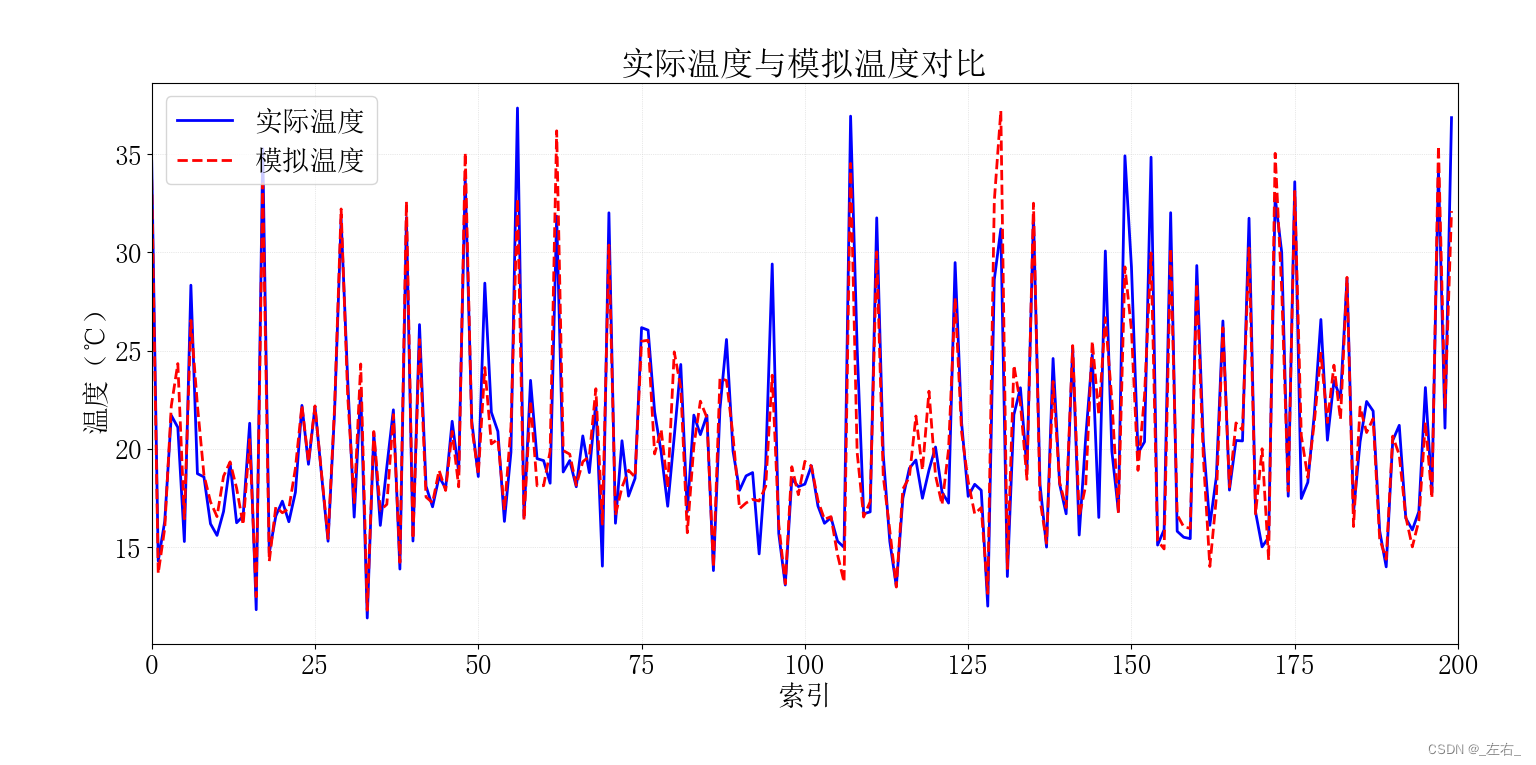
plt.plot(test_index_subset, y_test_subset, label='实际温度', color='blue', linewidth=2)
plt.plot(test_index_subset, y_pred_subset, label='模拟温度', color='red', linestyle='--', linewidth=2)
plt.title('实际温度与模拟温度对比')
plt.xlabel('索引')
plt.ylabel('温度（℃）')
plt.xlim(0, subset_size)
plt.legend()
plt.grid(color='lightgray', linestyle=':', linewidth=0.5, axis='both')
plt.tight_layout()
plt.show()

# 保存scaler实例
with open(r'D:\a新模型代码\scaler.pkl', 'wb') as scaler_file:
    pickle.dump(scaler, scaler_file)
    
# 保存最终模型
with open(r'D:\a新模型代码\best_ridge_regression_model.pkl', 'wb') as file:
    pickle.dump(best_ridge, file)

print("优化后的模型已保存至D:\新模型代码\best_ridge_regression_model.pkl")

输出样例：

可视化结果：

模型调用：

import pandas as pd
import numpy as np
from sklearn.preprocessing import MinMaxScaler
import pickle
from sklearn.linear_model import Ridge  # 确保这里是Ridge模型
from sklearn.metrics import mean_squared_error, mean_absolute_error, r2_score

# 加载scaler
with open(r'D:\a新模型代码\scaler.pkl', 'rb') as scaler_file:
    scaler = pickle.load(scaler_file)

# 加载岭回归模型
with open(r'D:\a新模型代码\best_ridge_regression_model.pkl', 'rb') as file:  # 文件名应与你保存的岭回归模型文件名一致
    model = pickle.load(file)
    
# 导入新数据
new_data = pd.read_excel(r'D:\a新模型代码\测试数据.xlsx')  # 更改为新数据的实际路径

# 数据预处理 - 使用训练时的scaler进行缩放
new_data_scaled = scaler.transform(new_data[['湿度', 'CO2', '光照', '土壤温度', '土壤湿度']])

# 使用模型进行预测
predictions = model.predict(new_data_scaled)

# 打印预测结果
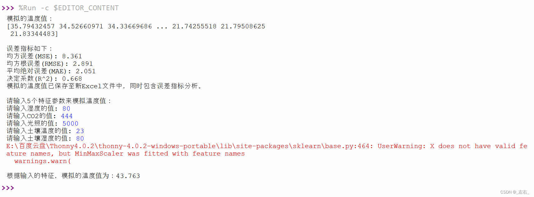
print("模拟的温度值：")
print(predictions)

# 将预测值添加到新数据框中作为一个新列
new_data['温度模拟值'] = predictions

# 如果新数据包含实际温度值，计算并打印误差指标
if '温度' in new_data.columns:
    mse = mean_squared_error(new_data['温度'], predictions)
    rmse = np.sqrt(mse)
    mae = mean_absolute_error(new_data['温度'], predictions)
    r2 = r2_score(new_data['温度'], predictions)

    print("\n误差指标如下：")
    print(f"均方误差(MSE): {mse:.3f}")
    print(f"均方根误差(RMSE): {rmse:.3f}")
    print(f"平均绝对误差(MAE): {mae:.3f}")
    print(f"决定系数(R^2): {r2:.3f}")

    # 保存新数据到Excel，包含预测值
    output_path = r'D:\a新模型代码\测试数据_岭回归模拟值.xlsx'
    new_data.to_excel(output_path, index=False)
    print("模拟的温度值已保存至新Excel文件中，同时包含误差指标分析。")
else:
    print("警告：新数据中未找到'温度'列，无法计算误差。模拟值已保存但无误差分析。")
    output_path = r'D:\a新模型代码\测试数据_岭回归模拟值.xlsx'
    new_data.to_excel(output_path, index=False)
    print("模拟的温度值已保存至新Excel文件中。")

# 手动输入特征进行预测
print("\n请输入5个特征参数来模拟温度值：")
feature_names = ['湿度', 'CO2', '光照', '土壤温度', '土壤湿度']
manual_features = []

for name in feature_names:
    value = float(input(f"请输入{name}的值: "))
    manual_features.append(value)

# 转换为numpy数组以便进行预测
manual_features_array = np.array([manual_features])

# 需要使用训练时使用的scaler对输入特征进行相同的预处理
manual_features_scaled = scaler.transform(manual_features_array)

# 预测
predicted_temp = model.predict(manual_features_scaled)

print(f"\n根据输入的特征，模拟的温度值为：{predicted_temp[0]:.3f}")

输出样例：