


用粒子群优化库pyswarms搜索LSTM模型最优超参数:神经元数量、激活函数、批量
import pandas as pd # 导入pandas模块,用于数据处理和分析
from math import sqrt # 从math模块导入sqrt函数,用于计算平方根
import matplotlib.pyplot as plt # 导入matplotlib.pyplot模块,用于绘图
import numpy as np # 导入numpy模块,用于数值计算
from sklearn.preprocessing import MinMaxScaler # 导入sklearn中的MinMaxScaler,用于特征缩放
from tensorflow.keras.layers import * # 从tensorflow.keras.layers导入所有层,用于构建神经网络
from tensorflow.keras.models import * # 从tensorflow.keras.models导入所有模型,用于构建和管理模型
from sklearn.metrics import mean_squared_error, mean_absolute_error, r2_score # 导入额外的评估指标
from tensorflow.keras import Input, Model, Sequential # 从tensorflow.keras导入Input, Model和Sequential,用于模型构建
import warnings
import pickle
from prettytable import PrettyTable # 可以优美的打印表格结果
from tensorflow.keras.utils import plot_model # 导入plot_model函数,用于绘制模型结构图
from tensorflow.keras.optimizers import Adam
import pyswarms as ps
from tensorflow.keras.callbacks import EarlyStopping
import time
warnings.filterwarnings("ignore") # 取消警告
plt.figure(figsize=(10, 6))
plt.rcParams['font.sans-serif'] = ['SimSun'] # 设置中文字体为宋体
plt.rcParams['font.serif'] = ['Times New Roman'] # 设置英文字体为新罗马
plt.rcParams['axes.unicode_minus'] = False # 解决保存图像是负号'-'显示为方块的问题
plt.rcParams['font.size'] = 20 # 设置字体大小
dataset = pd.read_excel('数据加室外天气.xlsx')
print(dataset) # 显示dataset数据
# 单输入单步预测,就让values等于某一列数据,n_out = 1,n_in, num_samples, scroll_window 根据自己情况来
# 单输入多步预测,就让values等于某一列数据,n_out > 1,n_in, num_samples, scroll_window 根据自己情况来
# 多输入单步预测,就让values等于多列数据,n_out = 1,n_in, num_samples, scroll_window 根据自己情况来
# 多输入多步预测,就让values等于多列数据,n_out > 1,n_in, num_samples, scroll_window 根据自己情况来
values = dataset.values[:, 1:] # 只取第2列数据,要写成1:2;只取第3列数据,要写成2:3,取第2列之后(包含第二列)的所有数据,写成 1:
# 从dataset DataFrame中提取数据。
# dataset.values将DataFrame转换为numpy数组。
# [:,1:]表示选择所有行(:)和从第二列到最后一列(1:)的数据。
# 这样做通常是为了去除第一列,这在第一列是索引或不需要的数据时很常见。
# 确保所有数据是浮动的
values = values.astype('float32')
# 将values数组中的数据类型转换为float32。
# 这通常用于确保数据类型的一致性,特别是在准备输入到神经网络模型中时。
def data_collation(data, n_in, n_out, or_dim, scroll_window, num_samples):
res = np.zeros((num_samples, n_in * or_dim + n_out))
for i in range(0, num_samples):
h1 = values[scroll_window * i: n_in + scroll_window * i, 0:or_dim]
h2 = h1.reshape(1, n_in * or_dim)
h3 = values[n_in + scroll_window * (i): n_in + scroll_window * (i) + n_out, -1].T
h4 = h3[np.newaxis, :]
h5 = np.hstack((h2, h4))
res[i, :] = h5
return res
# In[7]:
# 这里来个多特征输入,单步预测的案例
n_in = 72 # 输入前5行的数据
n_out = 6 # 预测未来2步的数据
or_dim = values.shape[1] # 记录特征数据维度
num_samples = len(values) - n_in - n_out + 1 # 可以设定从数据中取出多少个点用于本次网络的训练与测试。
scroll_window = 1 # 如果等于1,下一个数据从第二行开始取。如果等于2,下一个数据从第三行开始取
res = data_collation(values, n_in, n_out, or_dim, scroll_window, num_samples)
# 把数据集分为训练集和测试集
values = np.array(res)
# 将前面处理好的DataFrame(data)转换成numpy数组,方便后续的数据操作。
n_train_number = int(num_samples * 0.80)
# 计算训练集的大小。
# 设置80%作为训练集
# int(...) 确保得到的训练集大小是一个整数。
# 先划分数据集,在进行归一化,这才是正确的做法!
Xtrain = values[:n_train_number, :n_in * or_dim]
Ytrain = values[:n_train_number, n_in * or_dim:]
Xtest = values[n_train_number:, :n_in * or_dim]
Ytest = values[n_train_number:, n_in * or_dim:]
# 对训练集和测试集进行归一化
m_in = MinMaxScaler()
vp_train = m_in.fit_transform(Xtrain) # 注意fit_transform() 和 transform()的区别
vp_test = m_in.transform(Xtest) # 注意fit_transform() 和 transform()的区别
m_out = MinMaxScaler()
vt_train = m_out.fit_transform(Ytrain) # 注意fit_transform() 和 transform()的区别
vt_test = m_out.transform(Ytest) # 注意fit_transform() 和 transform()的区别
vp_train = vp_train.reshape((vp_train.shape[0], n_in, or_dim))
# 将训练集的输入数据vp_train重塑成三维格式。
# 结果是一个三维数组,其形状为[样本数量, 时间步长, 特征数量]。
vp_test = vp_test.reshape((vp_test.shape[0], n_in, or_dim))
# 将训练集的输入数据vp_test重塑成三维格式。
# 结果是一个三维数组,其形状为[样本数量, 时间步长, 特征数量]。
from keras.layers import Dense, Activation, Dropout, LSTM, Bidirectional, LayerNormalization, Input
from tensorflow.keras.models import Model
from sklearn.model_selection import KFold
def create_model(params):
n_batch, n_neurons_1, activation_1_idx, n_neurons_2, activation_2_idx = params
# 将整数索引转换为激活函数字符串
activation_1 = ['relu', 'tanh', 'sigmoid', 'selu'][int(activation_1_idx)]
activation_2 = ['relu', 'tanh', 'sigmoid', 'selu'][int(activation_2_idx)]
inputs = Input(shape=(vp_train.shape[1], vp_train.shape[2]))
lstm1 = LSTM(int(n_neurons_1), activation=activation_1, return_sequences=True)(inputs)
dropout1 = Dropout(rate=0.2)(lstm1)
lstm2 = LSTM(int(n_neurons_2), activation=activation_2, return_sequences=False)(dropout1)
dropout2 = Dropout(rate=0.2)(lstm2)
outputs = Dense(vt_train.shape[1])(dropout2)
model = Model(inputs=inputs, outputs=outputs)
optimizer = Adam(learning_rate=0.001)
model.compile(loss='mse', optimizer=optimizer)
return model
def evaluate_model(params):
model = create_model(params)
early_stopping = EarlyStopping(monitor='val_loss', patience=10, restore_best_weights=True)
history = model.fit(vp_train, vt_train, batch_size=int(params[0]), epochs=50, validation_split=0.2, verbose=0,
callbacks=[early_stopping])
y_pred = model.predict(vp_test)
mse = mean_squared_error(vt_test, y_pred)
return mse
def objective_function(x):
n_particles = x.shape[0]
losses = np.zeros(n_particles)
for i in range(n_particles):
params = x[i]
losses[i] = evaluate_model(params)
return losses
# 定义超参数的搜索范围,学习因子、惯性权重
options = {'c1': 0.5, 'c2': 0.3, 'w': 0.9}
# 定义超参数的边界
# [batch_size, neurons_1, activation_1_idx, neurons_2, activation_2_idx, learning_rate]
# 激活函数用整数表示,例如:0: 'relu', 1: 'tanh', 2: 'sigmoid', 3: 'selu'
bounds = (np.array([16, 16, 0, 16, 0]), np.array([64, 64, 3, 128, 3]))
# 创建PSO优化器
optimizer = ps.single.GlobalBestPSO(n_particles=10, dimensions=5, options=options, bounds=bounds)
# 测量运行时间
start_time = time.time()
# 运行优化
cost, pos = optimizer.optimize(objective_function, iters=20)
# 计算运行时间
end_time = time.time()
elapsed_time = end_time - start_time
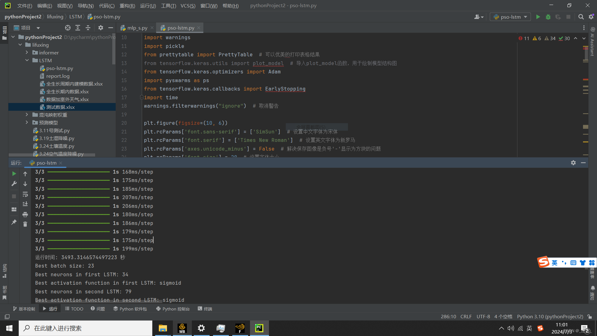
print(f"运行时间: {elapsed_time} 秒")
# 解析最佳超参数
best_batch_size = int(pos[0])
best_neurons_1 = int(pos[1])
best_activation_1_idx = int(pos[2])
best_neurons_2 = int(pos[3])
best_activation_2_idx = int(pos[4])
# 将整数索引转换为激活函数字符串
best_activation_1 = ['relu', 'tanh', 'sigmoid', 'selu'][best_activation_1_idx]
best_activation_2 = ['relu', 'tanh', 'sigmoid', 'selu'][best_activation_2_idx]
print(f"Best batch size: {best_batch_size}")
print(f"Best neurons in first LSTM: {best_neurons_1}")
print(f"Best activation function in first LSTM: {best_activation_1}")
print(f"Best neurons in second LSTM: {best_neurons_2}")
print(f"Best activation function in second LSTM: {best_activation_2}")
# 使用最佳超参数构建和训练模型
best_params = [best_batch_size, best_neurons_1, best_activation_1_idx, best_neurons_2, best_activation_2_idx]
model = create_model(best_params)
early_stopping = EarlyStopping(monitor='val_loss', patience=10, restore_best_weights=True)
history = model.fit(vp_train, vt_train, batch_size=best_batch_size, epochs=200, validation_split=0.2, verbose=2,
callbacks=[early_stopping])
# 绘制历史数据
plt.plot(history.history['loss'], label='Training Loss')
plt.plot(history.history['val_loss'], label='Validation Loss')
plt.legend()
plt.xlabel("Epochs")
plt.ylabel("Loss")
plt.show()
# 作出预测
yhat = model.predict(vp_test)
# 使用模型对测试集的输入特征(vp_test)进行预测。
# yhat是模型预测的输出值。
yhat = yhat.reshape(num_samples - n_train_number, n_out)
# 将预测值yhat重塑为二维数组,以便进行后续操作。
predicted_data = m_out.inverse_transform(yhat) # 反归一化
def mape(y_true, y_pred):
# 定义一个计算平均绝对百分比误差(MAPE)的函数。
record = []
for index in range(len(y_true)):
# 遍历实际值和预测值。
temp_mape = np.abs((y_pred[index] - y_true[index]) / y_true[index])
record.append(temp_mape)
return np.mean(record) * 100
def evaluate_forecasts(Ytest, predicted_data, n_out):
# 定义一个函数来评估预测的性能。
mse_dic = []
rmse_dic = []
mae_dic = []
mape_dic = []
r2_dic = []
# 初始化存储各个评估指标的字典。
table = PrettyTable(['测试集指标', 'MSE', 'RMSE', 'MAE', 'MAPE', 'R2'])
for i in range(n_out):
# 遍历每一个预测步长。每一列代表一步预测,现在是在求每步预测的指标
actual = [float(row[i]) for row in Ytest] # 一列列提取
# 从测试集中提取实际值。
predicted = [float(row[i]) for row in predicted_data]
# 从预测结果中提取预测值。
mse = mean_squared_error(actual, predicted)
# 计算均方误差(MSE)。
mse_dic.append(mse)
rmse = sqrt(mean_squared_error(actual, predicted))
# 计算均方根误差(RMSE)。
rmse_dic.append(rmse)
mae = mean_absolute_error(actual, predicted)
# 计算平均绝对误差(MAE)。
mae_dic.append(mae)
MApe = mape(actual, predicted)
# 计算平均绝对百分比误差(MAPE)。
mape_dic.append(MApe)
r2 = r2_score(actual, predicted)
# 计算R平方值(R2)。
r2_dic.append(r2)
if n_out == 1:
strr = '预测结果指标:'
else:
strr = '第' + str(i + 1) + '步预测结果指标:'
table.add_row([strr, mse, rmse, mae, str(MApe) + '%', str(r2 * 100) + '%'])
return mse_dic, rmse_dic, mae_dic, mape_dic, r2_dic, table
# 返回包含所有评估指标的字典。
mse_dic, rmse_dic, mae_dic, mape_dic, r2_dic, table = evaluate_forecasts(Ytest, predicted_data, n_out)
print(table) # 显示预测指标数值
## 画结果图
from matplotlib import rcParams
plt.ion()
for ii in range(n_out):
plt.figure(figsize=(10, 6))
x = range(1, len(predicted_data) + 1)
interval = max(1, len(x) // 10) # 自动计算合适的间隔
plt.xticks(x[::interval]) # 显示刻度并旋转标签
plt.tick_params(labelsize=15) # 改变刻度字体大小
plt.plot(x, predicted_data[:, ii], linestyle="--", linewidth=1, label='预测值')
plt.plot(x, Ytest[:, ii], linestyle="-", linewidth=1, label='真实值')
plt.rcParams.update({'font.size': 15}) # 改变图例里面的字体大小
# 更新图例的字体大小。
plt.legend(loc='best', )
plt.xlabel("时间步长", )
plt.ylabel("温度(℃)", )
plt.ioff() # 关闭交互模式
plt.show()
scaler_path1 = 'scaler1.pkl'
with open(scaler_path1, 'wb') as scaler_file:
pickle.dump(m_in, scaler_file)
scaler_path2 = 'scaler2.pkl'
with open(scaler_path2, 'wb') as scaler_file:
pickle.dump(m_out, scaler_file)
model.save(r'D:aa\saved_model.h5') # 保存模型到指定路径
结果:


 1万+
1万+

 被折叠的 条评论
为什么被折叠?
被折叠的 条评论
为什么被折叠?
 到【灌水乐园】发言


