深度学习实战05-卷积神经网络（CNN）实现彩色图片分类

​
​

活动地址：CSDN21天学习挑战赛
参考文章：https://mtyjkh.blog.csdn.net/article/details/116978213

一、前期工作

1. 设置GPU

import tensorflow as tf
gpus = tf.config.list_physical_devices("GPU")

if gpus:
    gpu0 = gpus[0] #如果有多个GPU，仅使用第0个GPU
    tf.config.experimental.set_memory_growth(gpu0, True) #设置GPU显存用量按需使用
    tf.config.set_visible_devices([gpu0],"GPU")

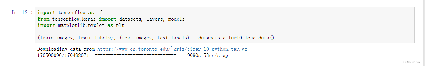
2. 导入数据

import tensorflow as tf
from tensorflow.keras import datasets, layers, models
import matplotlib.pyplot as plt

(train_images, train_labels), (test_images, test_labels) = datasets.cifar10.load_data()

3. 归一化

# 将像素的值标准化到0-1的区间。
train_images, test_images = train_images / 255.0, test_images / 255.0

train_images.shape, test_images.shape, train_labels.shape, test_labels.shape

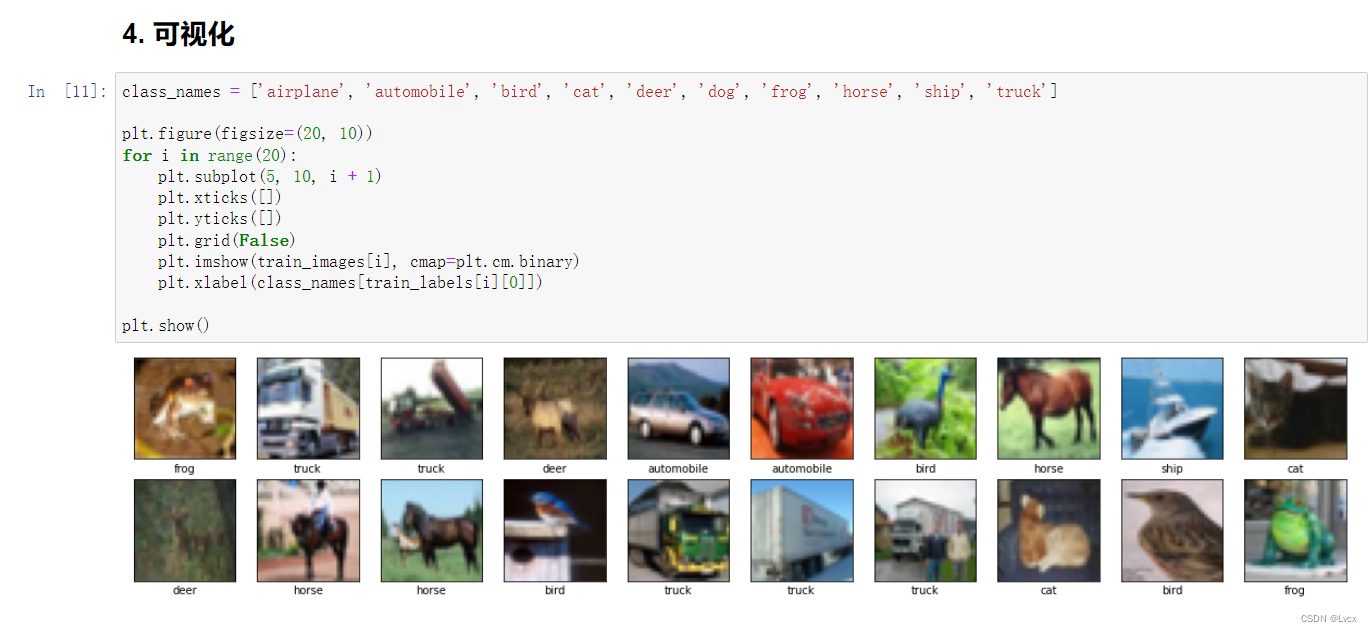
4. 可视化

class_names = ['airplane', 'automobile', 'bird', 'cat', 'deer', 'dog', 'frog', 'horse', 'ship', 'truck']

plt.figure(figsize=(20, 10))
for i in range(20):
    plt.subplot(5, 10, i + 1)
    plt.xticks([])
    plt.yticks([])
    plt.grid(False)
    plt.imshow(train_images[i], cmap=plt.cm.binary)
    plt.xlabel(class_names[train_labels[i][0]])

plt.show()    

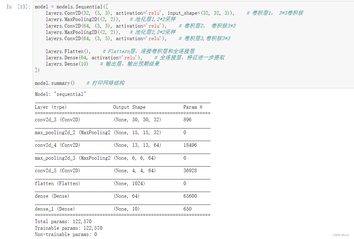
二、构建CNN网络

model = models.Sequential([
    layers.Conv2D(32, (3, 3), activation='relu', input_shape=(32, 32, 3)),    # 卷积层1， 3*3卷积核
    layers.MaxPooling2D((2, 2)),   # 池化层1,2*2采样
    layers.Conv2D(64, (3, 3), activation='relu'),    # 卷积层2， 卷积核3*3
    layers.MaxPooling2D((2, 2)),   # 池化层2,2*2采样
    layers.Conv2D(64, (3, 3), activation='relu'),    # 卷积层3,卷积核3*3
   
    layers.Flatten(),    # Flattern层，连接卷积层和全连接层
    layers.Dense(64, activation='relu'),    # 全连接层，特征进一步提取
    layers.Dense(10)    # 输出层，输出预期结果
])

model.summary()    # 打印网络结构

三、编译

model.compile(optimizer='adam',
             loss=tf.keras.losses.SparseCategoricalCrossentropy(from_logits=True),
             metrics=['accuracy'])

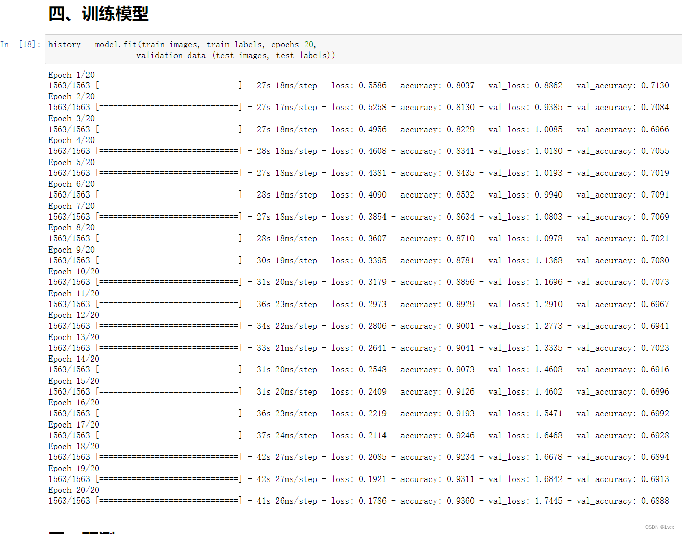
四、训练模型

history = model.fit(train_images, train_labels, epochs=20,
                   validation_data=(test_images, test_labels))

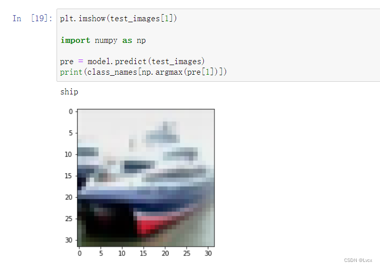
五、预测

通过模型进行预测得到的是每一个类别的概率，数字越大该图片为该类别的可能性越大。

plt.imshow(test_images[1])

import numpy as np

pre = model.predict(test_images)
print(class_names[np.argmax(pre[1])])

六、模型评估

import matplotlib.pyplot as plt

plt.plot(history.history['accuracy'], label='accuracy')
plt.plot(history.history['val_accuracy'], label='val_accuracy')
plt.xlabel('Epoch')
plt.ylabel('Accuracy')
plt.ylim([0.5, 1])
plt.legend(loc='lower right')
plt.show()

test_loss, test_acc = model.evaluate(test_images, test_labels, verbose=2)

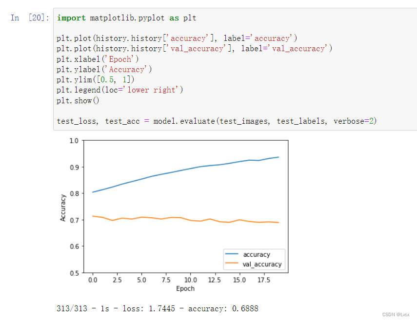
print(test_acc)

​