


📈 基于 LSTM 的时间序列预测模型实战(含完整代码、可视化与多组超参数调优)
在时间序列预测中,LSTM(Long Short-Term Memory)因其处理时序信息的能力被广泛应用于金融预测、气象分析、位移监测等领域。本文将带你一步步搭建一个完整的 LSTM 时间序列预测系统:从数据预处理、模型设计,到训练可视化、预测评估,全流程覆盖。
本项目结合 CSDN 博客《【时间序列预测03】-LSTM 长短期记忆网络(Long Short-Term Memory) 》中关于 MLP 的基础知识,以一个包含两个特征变量的时序数据集为例,搭建一个自动化的训练评估流程,从数据加载、预处理、模型训练到预测评估与结果可视化,全部实现自动保存、自动记录。 适合对 LSTM、深度学习在时间序列中的应用感兴趣的读者参考和实践。
🚀 项目亮点
- 🔁 多组超参数自动循环(filters、batch_size、learning_rate、look_back)
- 🧠 使用 Keras + TensorFlow 搭建 LSTM 网络,结构灵活可拓展
- 🧹 集成 EarlyStopping + ModelCheckpoint,避免过拟合并保存最优模型
- 📉 输出完整评估指标(MAE、RMSE、MAPE、R²)并保存至 CSV
- 📊 自动绘制并保存训练 loss 曲线与预测结果图像
- 📁 项目结构清晰,便于组织与管理不同配置下的结果
📌 使用说明
- 准备数据集:将你的数据存为 CSV 文件,包含
date和至少两个数值型特征(可修改支持更多维度) - 修改路径:将
df = read_csv('../data/df.csv')替换为你的数据路径 - 设置参数:可根据需要调整
n_features,hours_train,filters,look_back等 - 运行
lstm_train.py脚本,程序将自动遍历各组超参数并保存模型、图像和指标
一、导入所需要的库
import pandas as pd
import matplotlib.pyplot as plt
from numpy import concatenate
from sklearn.preprocessing import MinMaxScaler, LabelEncoder
from sklearn.metrics import mean_squared_error, mean_absolute_error, mean_absolute_percentage_error, r2_score
from keras.models import Sequential
from keras.layers import Dense, Flatten,LSTM
import matplotlib as mpl
import tensorflow as tf
from pandas import read_csv
from math import sqrt
from tensorflow.keras.layers import Input
import os
import random
import numpy as np
TimeSeriesSupervised 是一个专为时间序列数据转换为监督学习问题而设计的工具类。它将时间序列数据转换为可以用于机器学习模型训练的输入输出对,常用于时间序列预测任务。
from sklearn.base import BaseEstimator, TransformerMixin

class TimeSeriesSupervised(BaseEstimator, TransformerMixin):
    """
    Convert a time series dataset into a supervised learning format.
    """
    def __init__(self, look_back=1, predict_forward=1, dropnan=True):
        self.look_back = look_back
        self.predict_forward = predict_forward
        self.dropnan = dropnan

    def fit(self, X, y=None):
        return self

    def transform(self, X):
        if isinstance(X, pd.DataFrame):
            data = X.values
        elif isinstance(X, np.ndarray):
            data = X
        else:
            raise ValueError("Input must be a NumPy array or a pandas DataFrame.")

        n_vars = 1 if len(data.shape) == 1 else data.shape[1]
        df = pd.DataFrame(data)
        cols, names = list(), list()

        # input sequence (t-n, ... t-1)
        for i in range(self.look_back, 0, -1):
            cols.append(df.shift(i))
            names += [f'var{j+1}(t-{i})' for j in range(n_vars)]

        # forecast sequence (t, t+1, ... t+n)
        for i in range(0, self.predict_forward):
            cols.append(df.shift(-i))
            if i == 0:
                names += [f'var{j+1}(t)' for j in range(n_vars)]
            else:
                names += [f'var{j+1}(t+{i})' for j in range(n_vars)]

        # put it all together
        agg = pd.concat(cols, axis=1)
        agg.columns = names

        # drop rows with NaN values
        if self.dropnan:
            agg.dropna(inplace=True)

        return agg
可重复性控制(随机种子)
要让你的代码每次运行时结果一致,可以设置**随机种子(random seed)**来控制各种涉及随机性的部分。你已经在用 TensorFlow、Keras、NumPy 等库,所以需要为这些库分别设定随机种子。
# 设置PYTHONHASHSEED环境变量
os.environ['PYTHONHASHSEED'] = '42'

# Python内置random模块的随机种子
random.seed(42)

# NumPy的随机种子
np.random.seed(42)

# TensorFlow的随机种子
tf.random.set_seed(42)
简单地判断是否启用了 GPU
physical_devices = tf.config.experimental.list_physical_devices('GPU')
for device in physical_devices:
    tf.config.experimental.set_memory_growth(device, True)
print("Num GPUs Available: ", len(tf.config.experimental.list_physical_devices('GPU')))
Num GPUs Available: 0
关闭图表中坐标轴(axes)的默认网格线(grid)显示。
mpl.rcParams['axes.grid'] = False
二、加载数据
读取并预处理你的时间序列数据
把 date 这一列设置为 索引列,使得你的 DataFrame 变成时间索引结构(即:时间序列格式);
df = read_csv('../data/df.csv')
df
| date | p5 | rain | |
|---|---|---|---|
| 0 | 2015-04-10 | 1.041892 | 12.4 |
| 1 | 2015-04-21 | 0.186168 | 34.0 |
| 2 | 2015-05-02 | -2.374851 | 31.6 |
| 3 | 2015-05-13 | 0.548328 | 62.4 |
| 4 | 2015-05-24 | -0.684310 | 8.2 |
| ... | ... | ... | ... |
| 156 | 2019-12-21 | -1.270302 | 20.8 |
| 157 | 2020-01-01 | 2.232585 | 26.8 |
| 158 | 2020-01-12 | 0.175435 | 1.8 |
| 159 | 2020-01-23 | -0.253113 | 61.0 |
| 160 | 2020-02-03 | 0.346710 | 39.6 |
161 rows × 3 columns
dataset = df.set_index('date')
dataset
| p5 | rain | |
|---|---|---|
| date | ||
| 2015-04-10 | 1.041892 | 12.4 |
| 2015-04-21 | 0.186168 | 34.0 |
| 2015-05-02 | -2.374851 | 31.6 |
| 2015-05-13 | 0.548328 | 62.4 |
| 2015-05-24 | -0.684310 | 8.2 |
| ... | ... | ... |
| 2019-12-21 | -1.270302 | 20.8 |
| 2020-01-01 | 2.232585 | 26.8 |
| 2020-01-12 | 0.175435 | 1.8 |
| 2020-01-23 | -0.253113 | 61.0 |
| 2020-02-03 | 0.346710 | 39.6 |
161 rows × 2 columns
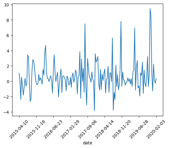
可视化位移数据
# plot displacement
dataset['p5'].plot()
plt.xticks(rotation=45)
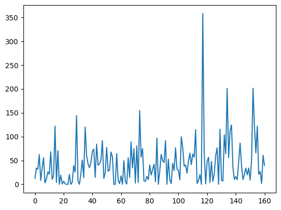
# plot rain
df['rain'].plot()
查看每个变量的统计特征(均值、最大值、标准差等)
# statistics of the dataset
dataset.describe().transpose()
| count | mean | std | min | 25% | 50% | 75% | max | |
|---|---|---|---|---|---|---|---|---|
| p5 | 161.0 | 0.634245 | 2.032216 | -3.847115 | -0.467202 | 0.381206 | 1.214105 | 9.427837 |
| rain | 161.0 | 43.162733 | 46.266452 | 0.000000 | 9.400000 | 34.000000 | 62.400000 | 357.800000 |
hours_train = 100
表示用于训练模型的时间步长度是 100 个样本点(可能是小时、天,取决于数据的时间单位)。
n_features = 2
表示你的数据有 两个变量(或特征) —— 比如可能是 p5(位移) 和 rain。
# DEFINE TRAINING LENGHT (the remaining will be test)

#training hours
hours_train=100

# total number of variables
n_features = 2
# number of filters/nodes
filters = 16
# learning rates
lr = 5e-3
# epochs
epochs = 1000
# batch sizes
batch_size = 9
# how many time steps back do we want the model to see
look_backs = 3
三、数据预处理
3.1 时间序列转监督学习格式
look = look_backs

# load dataset
values = dataset.values
# ensure all data is float
values = values.astype('float32')
# normalize features
scaler = MinMaxScaler(feature_range=(0, 1))
scaled = scaler.fit_transform(values)
# specify the number of lag hours
n_hours = look
# frame as supervised learning

transformer = TimeSeriesSupervised(look_back=n_hours, predict_forward=1)
reframed = transformer.fit_transform(scaled)
print(reframed.shape)
(158, 8)
3.2. 划分数据集
# split into train and test sets
values = reframed.values
n_train_hours = hours_train - look
train = values[:n_train_hours, :]
test = values[n_train_hours:, :]
# split into input and outputs
n_obs = n_hours * n_features
train_X, train_y = train[:, :n_obs], train[:, -n_features]
test_X, test_y = test[:, :n_obs], test[:, -n_features]
print(train_X.shape, len(train_X), train_y.shape)
(97, 6) 97 (97,)
3.3 将输入数据重塑为 3D 数组
# reshape input to be 3D [samples, timesteps, features]
train_X = train_X.reshape((train_X.shape[0], n_hours, n_features))
test_X = test_X.reshape((test_X.shape[0], n_hours, n_features))
print(train_X.shape, train_y.shape, test_X.shape, test_y.shape)

n = - n_features + 1
(97, 3, 2) (97,) (61, 3, 2) (61,)
四、构建模型
4.1 定义模型
def LSTM_net(filters, lr):
    model = Sequential()
    model.add(Input(shape=(train_X.shape[1], train_X.shape[2])))  # 推荐用法
    model.add(LSTM(filters, return_sequences=False))              # 不需要 input_shape 参数
    model.add(Dense(1))
    model.compile(
        loss=tf.losses.Huber(),
        optimizer=tf.optimizers.Adam(learning_rate=lr),
        metrics=[tf.metrics.MeanAbsoluteError(), tf.metrics.MeanSquaredError()]
    )
    return model
这段代码是构建 LSTM 网络结构的函数 LSTM_net(filters, lr),意思是:根据你指定的超参数 filters(神经元数量)和 lr(学习率),生成一个LSTM模型。
我们逐行拆解它的意思,配点注释给你讲清楚👇:
def LSTM_net(filters, lr):
定义一个函数,输入两个参数:
filters:LSTM 层中的神经元个数(控制模型容量)lr:学习率(控制优化器的更新步长)
model = Sequential()
创建一个 Keras 的顺序模型(Sequential),适合像这样一层接一层的神经网络结构。
model.add(Input(shape=(train_X.shape[1], train_X.shape[2]))) # 推荐用法
添加一个显式的 Input 层。
train_X.shape[1]是时间步长(look_back)train_X.shape[2]是特征数(n_features)
➡️ 你告诉模型,输入是一个 二维时间序列数据,每个样本形状是:(时间步数, 特征数)。
这是符合 Keras 推荐的做法,避免警告 Do not pass input_shape to layer...
model.add(LSTM(filters, return_sequences=False))
添加一个 LSTM 层:
filters是隐藏单元个数,比如 64 或 128;return_sequences=False表示只输出最后一个时间步的隐藏状态,适合做单步预测。
model.add(Dense(1))
添加一个 Dense(全连接)层,输出是 1 个值,对应你要预测的下一个点(单步预测)。
    model.compile(
        loss=tf.losses.Huber(),
        optimizer=tf.optimizers.Adam(learning_rate=lr),
        metrics=[tf.metrics.MeanAbsoluteError(), tf.metrics.MeanSquaredError()]
    )
- 用 Huber 损失(鲁棒性更好,不容易被异常值影响);
- 优化器用 Adam,学习率用你传进来的
lr; - 同时追踪两个评估指标:MAE 和 MSE,训练时会显示。
🎯 总结一下这个函数的作用:
它返回了一个结构如下的 LSTM 模型:
Input(shape=(time_steps, features))
  ↓
LSTM(units=filters)
  ↓
Dense(1)
适用于时间序列回归任务,预测未来一个数值。
结构简单,训练快,适合用于模型调参、超参搜索。
五、训练模型
fil= filters
learning_rate = lr
batch = batch_size

# load the model
model = LSTM_net(filters=fil, lr=learning_rate)
# Save the models only when validation loss decrease
early_stop = tf.keras.callbacks.EarlyStopping(monitor='val_loss',  # what is the metric to measure
                                              patience=20,
                                              # how many epochs to continue running the model after seeing an increase in val_loss
                                              restore_best_weights=True)  # update the model weights
model_checkpoint = tf.keras.callbacks.ModelCheckpoint(
    f'models/LSTM/weights/filters_{fil}_batch_size_{batch}_lr_{learning_rate}_look_back_{look}.weights.h5',
    monitor='val_loss', mode='min', verbose=0,
    save_best_only=True, save_weights_only=True) #Keras 的 ModelCheckpoint 回调被触发保存模型时,它会自动创建中间目录,包括你提供路径中的
# fit network
history = model.fit(train_X, train_y, epochs=epochs, batch_size=batch, validation_split=0.2, verbose=0,
                    shuffle=False, callbacks=[model_checkpoint, early_stop])
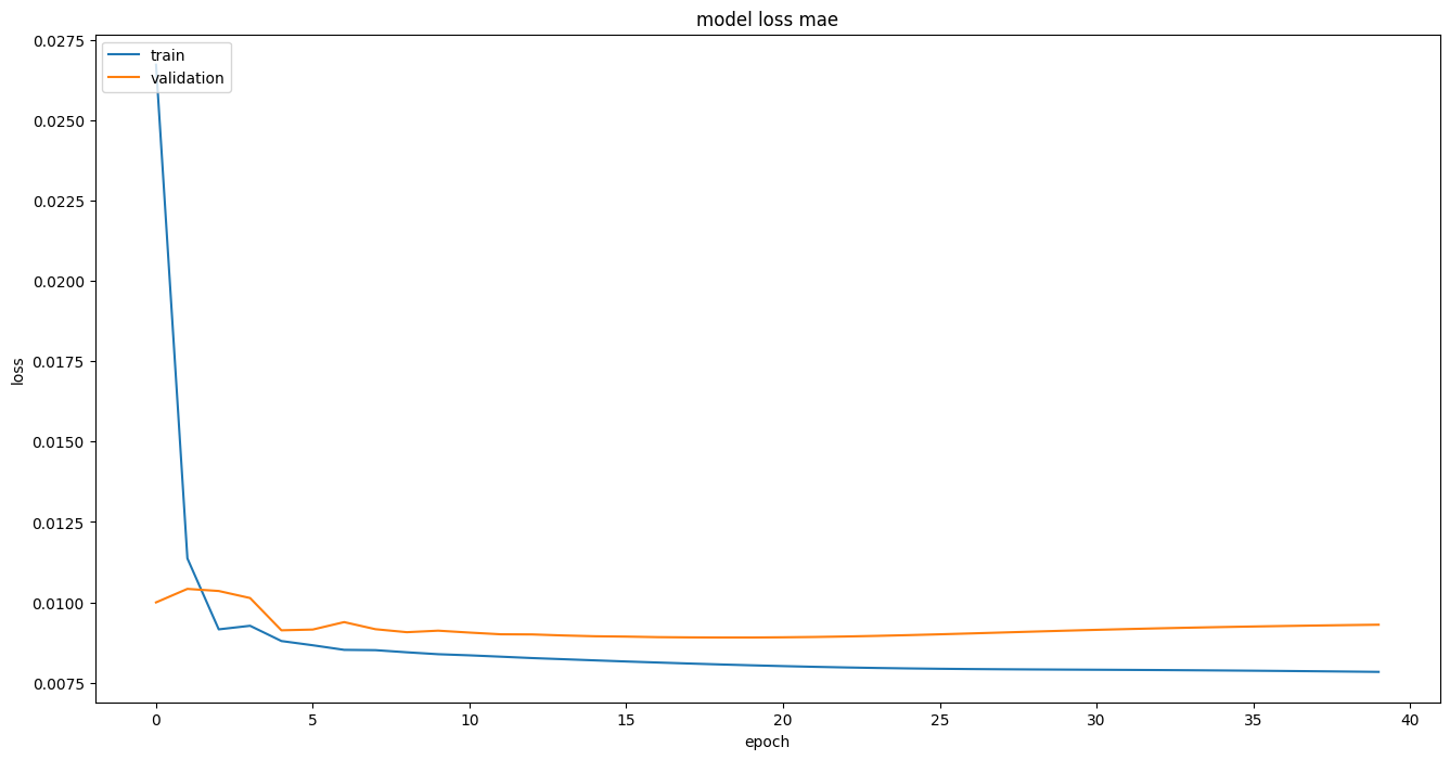
可视化loss
plt.figure(figsize=(16, 8))
plt.plot(history.history['loss'])
plt.plot(history.history['val_loss'])
plt.title('model loss mae')
plt.ylabel('loss')
plt.xlabel('epoch')
plt.legend(['train', 'validation'], loc='upper left')
六、预测
# load model to evaluate the test data
LSTM_model = LSTM_net(filters=fil, lr=learning_rate)
# load the last saved weight from the training
LSTM_model.load_weights(f"models/LSTM/weights/filters_{fil}_batch_size_{batch}_lr_{learning_rate}_look_back_{look}.weights.h5")

# Evaluate the model
yhat = LSTM_model.predict(test_X)
test_X_res = test_X.reshape((test_X.shape[0], n_hours * n_features))
# invert scaling for forecast
inv_yhat = concatenate((yhat, test_X_res[:, n:]), axis=1)
inv_yhat = scaler.inverse_transform(inv_yhat)
inv_yhat = inv_yhat[:, 0]
# invert scaling for actual
test_y = test_y.reshape((len(test_y), 1))
inv_y = concatenate((test_y, test_X_res[:, n:]), axis=1)
inv_y = scaler.inverse_transform(inv_y)
inv_y = inv_y[:, 0]
七、计算评估指标
# calculate MAE
mae = mean_absolute_error(inv_y, inv_yhat)
print('Test MAE: %.3f' % mae)
# calculate RMSE
rmse = sqrt(mean_squared_error(inv_y, inv_yhat))
print('Test RMSE: %.3f' % rmse)
# calculate MAPE
mape = mean_absolute_percentage_error(inv_y, inv_yhat)
print('Test MAPE: %.3f' % mape)
# calculate R2
r2 = r2_score(inv_y, inv_yhat)
print('Test R2: %.3f' % r2)
Test MAE: 1.517
Test RMSE: 2.290
Test MAPE: 2.182
Test R2: 0.125
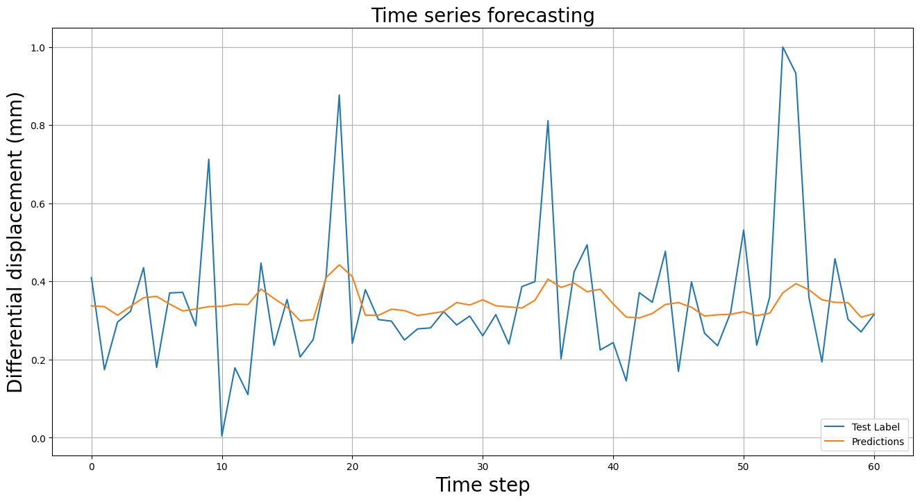
八、可视化预测结果
# 绘图
plt.figure(figsize=(16, 8))
plt.title('Time series forecasting', size=20)
plt.plot(pd.DataFrame(test_y), label='Test Label')
plt.plot(pd.DataFrame(yhat), label='Predictions')
plt.legend(loc='lower right', markerscale=1)
plt.xlabel('Time step', size=20)
plt.ylabel('Differential displacement (mm)', size=20)
plt.grid(True)
完整代码
import pandas as pd
import matplotlib.pyplot as plt
from numpy import concatenate
from sklearn.preprocessing import MinMaxScaler, LabelEncoder
from sklearn.metrics import mean_squared_error, mean_absolute_error, mean_absolute_percentage_error, r2_score
from keras.models import Sequential
from keras.layers import Dense, Flatten,LSTM
import matplotlib as mpl
import tensorflow as tf
from helper import *
from pandas import read_csv
from math import sqrt
from tensorflow.keras.layers import Input
import os
import random
import numpy as np
# 设置PYTHONHASHSEED环境变量
os.environ['PYTHONHASHSEED'] = '42'

# Python内置random模块的随机种子
random.seed(42)

# NumPy的随机种子
np.random.seed(42)

# TensorFlow的随机种子
tf.random.set_seed(42)

physical_devices = tf.config.experimental.list_physical_devices('GPU')
for device in physical_devices:
    tf.config.experimental.set_memory_growth(device, True)

mpl.rcParams['axes.grid'] = False


# 1. Load the dataset

df = read_csv('../data/df.csv')
dataset = df.set_index('date')

# 2. Preprocess the dataset
# DEFINE TRAINING LENGHT (the remaining will be test)

#training hours
hours_train=100

# total number of variables
n_features = 2

### LSTM ###


dic = {}

# number of filters/nodes
filters = [16, 32, 64, 96, 128, 256]
# learning rates
lr = [10e-3, 5e-3, 10e-4, 5e-4, 10e-5, 5e-5]
# epochs
epochs = 1000
# batch sizes
batch_size = [9, 18, 36, 72, 144]
# how many time steps back do we want the model to see
look_backs = [3, 5, 7, 9, 12]

# Hyperparameters
dic["batch_size"] = []
dic["learning_rate"] = []
dic["filters"] = []
dic["look_backs"] = []

# test_scores
dic["MAE"] = []
dic["RMSE"] = []
dic["MAPE"] = []
dic["R2"] = []

for fil in filters:
    for learning_rate in lr:
        for batch in batch_size:
            for look in look_backs:
                print('-------------------------------------------------------------------------------------')
                print('LSTM')
                print('Filters: ', fil)
                print('Learning rate: ', learning_rate)
                print('Batch size: ', batch)
                print('Look back: ', look)
                # load dataset
                values = dataset.values
                # ensure all data is float
                values = values.astype('float32')
                # normalize features
                scaler = MinMaxScaler(feature_range=(0, 1))
                scaled = scaler.fit_transform(values)
                # specify the number of lag hours
                n_hours = look
                # frame as supervised learning
                reframed = series_to_supervised(scaled, n_hours, 1)
                print(reframed.shape)

                # split into train and test sets
                values = reframed.values
                n_train_hours = hours_train - look
                train = values[:n_train_hours, :]
                test = values[n_train_hours:, :]
                # split into input and outputs
                n_obs = n_hours * n_features
                train_X, train_y = train[:, :n_obs], train[:, -n_features]
                test_X, test_y = test[:, :n_obs], test[:, -n_features]
                print(train_X.shape, len(train_X), train_y.shape)

                # reshape input to be 3D [samples, timesteps, features]
                train_X = train_X.reshape((train_X.shape[0], n_hours, n_features))
                test_X = test_X.reshape((test_X.shape[0], n_hours, n_features))
                print(train_X.shape, train_y.shape, test_X.shape, test_y.shape)

                n = - n_features + 1


                def LSTM_net(filters, lr):
                    model = Sequential()
                    model.add(LSTM(filters, return_sequences=False, input_shape=(train_X.shape[1], train_X.shape[2])))
                    model.add(Dense(1))
                    model.compile(loss=tf.losses.Huber(),
                                  optimizer=tf.optimizers.Adam(learning_rate=lr),
                                  metrics=[tf.metrics.MeanAbsoluteError(), tf.metrics.MeanSquaredError()])
                    model.summary()
                    return model


                # load the model
                model = LSTM_net(filters=fil, lr=learning_rate)
                # Save the models only when validation loss decrease
                early_stop = tf.keras.callbacks.EarlyStopping(monitor='val_loss',  # what is the metric to measure
                                                              patience=20,
                                                              # how many epochs to continue running the model after seeing an increase in val_loss
                                                              restore_best_weights=True)  # update the model weights
                model_checkpoint = tf.keras.callbacks.ModelCheckpoint(
                    f'models/LSTM/weights/filters_{fil}_batch_size_{batch}_lr_{learning_rate}_look_back_{look}.weights.h5',
                    monitor='val_loss', mode='min', verbose=0,
                    save_best_only=True, save_weights_only=True) #Keras 的 ModelCheckpoint 回调被触发保存模型时,它会自动创建中间目录,包括你提供路径中的
                # fit network
                history = model.fit(train_X, train_y, epochs=epochs, batch_size=batch, validation_split=0.2, verbose=0,
                                    shuffle=False, callbacks=[model_checkpoint, early_stop])

                plt.figure(figsize=(16, 8))
                plt.plot(history.history['loss'])
                plt.plot(history.history['val_loss'])
                plt.title('model loss mae')
                plt.ylabel('loss')
                plt.xlabel('epoch')
                plt.legend(['train', 'validation'], loc='upper left')

                # save plots


                # 创建保存目录
                save_path = 'models/LSTM/plots/'
                os.makedirs(save_path, exist_ok=True)

                # 保存图像
                filename = f"filters_{fil}_batch_size_{batch}_lr_{learning_rate}_look_back_{look}.png"
                plt.savefig(os.path.join(save_path, filename))#, facecolor='white', edgecolor='none', bbox_inches='tight'


                # plt.show()

                # load model to evaluate the test data
                LSTM_model = LSTM_net(filters=fil, lr=learning_rate)
                # load the last saved weight from the training
                LSTM_model.load_weights(f"models/LSTM/weights/filters_{fil}_batch_size_{batch}_lr_{learning_rate}_look_back_{look}.weights.h5")

                # Evaluate the model
                yhat = LSTM_model.predict(test_X)
                test_X_res = test_X.reshape((test_X.shape[0], n_hours * n_features))
                # invert scaling for forecast
                inv_yhat = concatenate((yhat, test_X_res[:, n:]), axis=1)
                inv_yhat = scaler.inverse_transform(inv_yhat)
                inv_yhat = inv_yhat[:, 0]
                # invert scaling for actual
                test_y = test_y.reshape((len(test_y), 1))
                inv_y = concatenate((test_y, test_X_res[:, n:]), axis=1)
                inv_y = scaler.inverse_transform(inv_y)
                inv_y = inv_y[:, 0]

                # calculate MAE
                mae = mean_absolute_error(inv_y, inv_yhat)
                print('Test MAE: %.3f' % mae)
                # calculate RMSE
                rmse = sqrt(mean_squared_error(inv_y, inv_yhat))
                print('Test RMSE: %.3f' % rmse)
                # calculate MAPE
                mape = mean_absolute_percentage_error(inv_y, inv_yhat)
                print('Test MAPE: %.3f' % mape)
                # calculate R2
                r2 = r2_score(inv_y, inv_yhat)
                print('Test R2: %.3f' % r2)

                # plot and save preds


                # 绘图
                plt.figure(figsize=(16, 8))
                plt.title('Time series forecasting', size=20)
                plt.plot(pd.DataFrame(test_y), label='Test Label')
                plt.plot(pd.DataFrame(yhat), label='Predictions')
                plt.legend(loc='lower right', markerscale=1)
                plt.xlabel('Time step', size=20)
                plt.ylabel('Differential displacement (mm)', size=20)
                plt.grid(True)

                # 自动创建保存目录(如果不存在)
                save_dir2 = 'models/LSTM/preds/'
                os.makedirs(save_dir2, exist_ok=True)
                # 构建文件名
                filename2 = f"filters_{fil}_batch_size_{batch}_lr_{learning_rate}_look_back_{look}.png"
                plt.savefig(os.path.join(save_dir2, filename2), facecolor='white', edgecolor='none', bbox_inches='tight')

                # 显示图像
                # plt.show()


                # save results on the dictionary
                dic["batch_size"].append(batch)
                dic["learning_rate"].append(learning_rate)
                dic["filters"].append(fil)
                dic["look_backs"].append(look)
                dic["MAE"].append(mae)
                dic["RMSE"].append(rmse)
                dic["MAPE"].append(mape)
                dic["R2"].append(r2)
                # Convert results to a dataframe
                results = pd.DataFrame(dic)
                # Export as csv

                # 自动创建保存目录
                results_dir = 'models/LSTM/results/'
                os.makedirs(results_dir, exist_ok=True)

                # 保存 CSV 文件
                results.to_csv(os.path.join(results_dir, 'LSTM_results.csv'), index=False)
                print('-------------------------------------------------------------------------------------')

print('LSTM finished!')
helper.py
from pandas import DataFrame, concat

# convert series to supervised learning
def series_to_supervised(data, n_in=1, n_out=1, dropnan=True):
    n_vars = 1 if type(data) is list else data.shape[1]
    df = DataFrame(data)
    cols, names = list(), list()
    # input sequence (t-n, ... t-1)
    for i in range(n_in, 0, -1):
        cols.append(df.shift(i))
        names += [('var%d(t-%d)' % (j + 1, i)) for j in range(n_vars)]
    # forecast sequence (t, t+1, ... t+n)
    for i in range(0, n_out):
        cols.append(df.shift(-i))
        if i == 0:
            names += [('var%d(t)' % (j + 1)) for j in range(n_vars)]
        else:
            names += [('var%d(t+%d)' % (j + 1, i)) for j in range(n_vars)]
    # put it all together
    agg = concat(cols, axis=1)
    agg.columns = names
    # drop rows with NaN values
    if dropnan:
        agg.dropna(inplace=True)
    return agg
数据集 链接


 4291
4291

 被折叠的 条评论
为什么被折叠?
被折叠的 条评论
为什么被折叠?
 到【灌水乐园】发言


