gan的几种变体_推荐系统系列第6部分,用于协作过滤的自动编码器的6种变体

gan的几种变体

RECSYS系列 (RECSYS SERIES)

Update: This article is part of a series where I explore recommendation systems in academia and industry. Check out the full series: Part 1, Part 2, Part 3, Part 4, Part 5, and Part 6.

更新: 本文是我探索学术界和行业推荐系统的系列文章的一部分。 查看完整的系列文章: 第1部分 第2部分 第3 部分 第4 部分 第5 部分 第6部分

Many recommendation models have been proposed during the last few years. However, they all have their limitations in dealing with data sparsity and cold-start issues.

在最近几年中已经提出了许多推荐模型。 但是,它们在处理数据稀疏性和冷启动问题方面都有其局限性。

  • The data sparsity occurs when the recommendation performance drops significantly if the interactions between users and items are very sparse.

    如果用户和项目之间的交互非常稀疏,则推荐性能显着下降时,就会发生数据稀疏

  • The cold-start issues occur when the model can’t recommend new users and new items.

    当模型无法推荐新用户和新项目时,就会出现冷启动问题

To solve these problems, recent approaches have exploited side information about users or items. However, the improvement of the recommendation performance is not significant due to the limitations of such models in capturing the user preferences and item features.

为了解决这些问题,最近的方法已经利用了有关用户或物品的辅助信息。 然而,由于这种模型在捕获用户偏好和项目特征方面的局限性,因此推荐性能的提高并不明显。

Auto-encoder is a type of neural network suited for unsupervised learning tasks, including generative modeling, dimensionality reduction, and efficient coding. It has shown its superiority in learning underlying feature representation in many domains, including computer vision, speech recognition, and language modeling. Given that knowledge, new recommendation architectures have incorporated autoencoder and thus brought more opportunities in re-inventing user experiences to satisfy customers.

自动编码器是一种神经网络,适用于无监督学习任务,包括生成建模,降维和有效编码。 它已显示出在许多领域中学习基础特征表示的优势,包括计算机视觉,语音识别和语言建模。 有了这些知识,新的推荐体系结构已合并了自动编码器,从而在重新发明用户体验以满足客户方面带来了更多机会。

  • While traditional models deal only with a single data source (rating or text), auto-encoder based models can handle heterogeneous data sources (rating, audio, visual, video).

    虽然传统模型仅处理单个数据源(评级或文本),但是基于自动编码器的模型可以处理异构数据源(评级,音频,视觉,视频)。

  • Auto-encoder has a better understanding of the user demands and item features, thus leading to higher recommendation accuracy than traditional models.

    自动编码器对用户需求和商品功能有更好的了解 ,因此比传统型号具有更高的推荐准确性。

  • Furthermore, auto-encoder helps the recommendation model to be more adaptable in multi-media scenarios and more effective in handling input noises than traditional models.

    此外,与传统模型相比,自动编码器可以帮助推荐模型在多媒体场景中更加适应 ,并在处理输入噪声方面更加有效。

In this post and those to follow, I will be walking through the creation and training of recommendation systems, as I am currently working on this topic for my Master Thesis.

在本博文以及后续博文中,我将逐步介绍推荐系统的创建和培训,因为我目前正在为我的硕士论文处理该主题。

  • Part 1 provided a high-level overview of recommendation systems, how to build them, and how they can be used to improve businesses across industries.

    第1部分概述了推荐系统,如何构建它们以及如何将其用于改善整个行业的业务。

  • Part 2 provided a careful review of the ongoing research initiatives concerning the strengths and application scenarios of these models.

    第2部分仔细审查了有关这些模型的优势和应用场景的正在进行的研究计划。

  • Part 3 provided a couple of research directions that might be relevant to the recommendation system scholar community.

    第3部分提供了一些与推荐系统学者社区有关的研究方向。

  • Part 4 provided the nitty-gritty mathematical details of 7 variants of matrix factorization that you can construct: ranging from the use of clever side features to the application of Bayesian methods.

    第4部分详细介绍了可以构造的7种矩阵分解的变体的数学细节:从使用巧妙的辅助功能到应用贝叶斯方法,不一而足。

  • Part 5 provided the architecture design of 5 variants of multi-layer perceptron based collaborative filtering models, which are discriminative models that can interpret the features in a non-linear fashion.

    第5部分提供了基于多层感知器的协作过滤模型的5种变体的体系结构设计,这些模型是可以以非线性方式解释特征的判别模型。

In Part 6, I explore the use of Auto-Encoders for collaborative filtering. More specifically, I will dissect six principled papers that incorporate Auto-Encoders into their recommendation architecture. But first, let’s walk through a primer on auto-encoder and its variants.

在第6部分中,我将探讨如何使用自动编码器进行协作过滤。 更具体地说,我将剖析六篇将自动编码器纳入其推荐体系结构的原理性论文。 但是首先,让我们逐步了解一下自动编码器及其变体。

自动编码器入门及其变体 (A Primer on Auto-encoder and Its Variants)

As illustrated in the diagram below, a vanilla auto-encoder consists of an input layer, a hidden layer, and an output layer. The input data is passed into the input layer. The input layer and the hidden layer constructs an encoder. The hidden layer and the output layer constructs a decoder. The output data comes out of the output layer.

如下图所示,香草自动编码器由输入层,隐藏层和输出层组成。 输入数据被传递到输入层。 输入层和隐藏层构成一个编码器。 隐藏层和输出层构成解码器。 输出数据来自输出层。

Image for post
Autoencoder Architecture
自动编码器架构

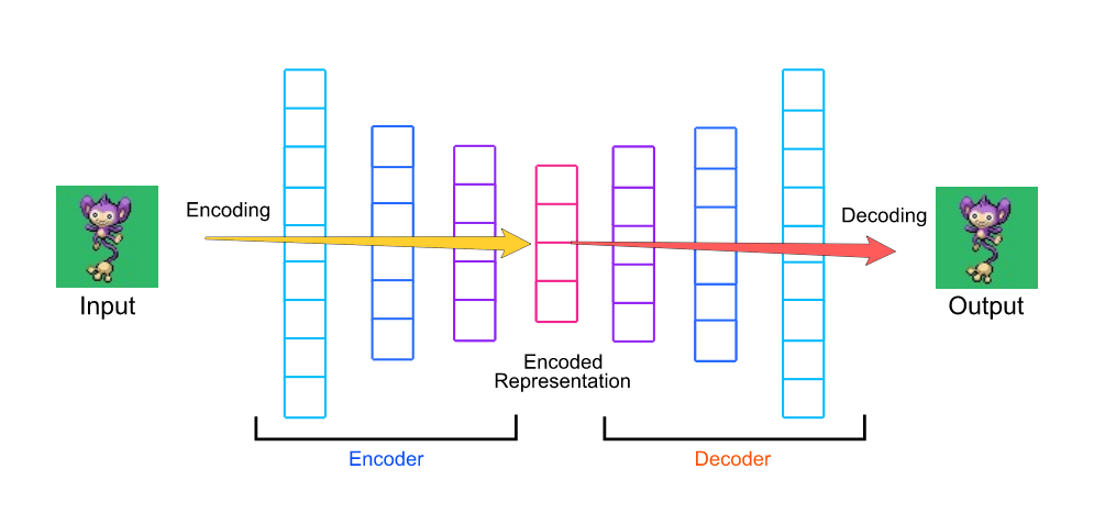
The encoder encodes the high-dimensional input data x into a lower-dimensional hidden representation h with a function f:

编码器使用函数f将高维输入数据x编码为低维隐藏表示h:

Image for post
Equation 1 等式1

where s_f is an activation function, W is the weight matrix, and b is the bias vector.

其中s_f是激活函数,W是权重矩阵,b是偏置矢量。

The decoder decodes the hidden representation h back to a reconstruction x’ by another function g:

解码器通过另一个函数g将隐藏的表示h解码回重建x':

Image for post
Equation 2
方程式2

where s_g is an activation function, W’ is the weight matrix, and b’ is the bias vector.

其中s_g是激活函数,W'是权重矩阵,b'是偏差矢量。

The choices of s_f and s_g are non-linear, for example, Sigmoid, TanH, or ReLU. This allows auto-encoder to learn more useful features than other unsupervised linear approaches, say Principal Component Analysis.

s_f和s_g的选择是非线性的,例如Sigmoid,TanH或ReLU。 主成分分析说,这使自动编码器比其他无监督线性方法学习更多有用的功能。

I can train the auto-encoder to minimize the reconstruction error between x and x’ via either the squared error (for regression tasks) or the cross-entropy error (for classification tasks).

我可以通过平方误差(对于回归任务)或交叉熵误差(对于分类任务)训练自动编码器,以最小化x和x'之间的重构误差。

This is the formula for the squared error:

这是平方误差的公式:

Image for post
Equation 3
方程式3

This is the formula for the cross-entropy error:

这是交叉熵误差的公式:

Image for post
Equation 4
方程式4

Finally, it is always a good practice to add a regularization term to the final reconstruction error of the auto-encoder:

最后,向自动编码器的最终重构错误中添加正则项始终是一个好习惯:

Image for post
Equation 5
方程式5

The reconstruction error function above can be optimized via either stochastic gradient descent or alternative least square.

上面的重建误差函数可以通过随机梯度下降或替代最小二乘法进行优化。

There are many variants of auto-encoders currently used in recommendation systems. The four most common are:

推荐系统中当前使用自动编码器的许多变体。 最常见的四个是:

  • Denoising Autoencoder (DAE) corrupts the inputs before mapping them into the hidden representation and then reconstructs the original input from its corrupted version. The idea is to force the hidden layer to acquire more robust features and to prevent the network from merely learning the identity function.

    去噪自动编码器(DAE)在将输入映射到隐藏表示之前先对其进行破坏,然后从其破坏的版本中重建原始输入。 这样做的目的是迫使隐藏层获得更强大的功能,并防止网络仅学习身份功能。

  • Stacked Denoising Autoencoder (SDAE) stacks several denoising auto-encoder on top of each other to get higher-level representations of the inputs. The training is usually optimized with greedy algorithms, going layer by layer. The apparent disadvantages here are the high computational cost of training and the lack of scalability to high-dimensional features.

    堆叠式去噪自动编码器(SDAE)彼此堆叠堆叠多个去噪自动编码器,以获得输入的更高级别表示。 训练通常使用贪心算法进行优化,并逐层进行。 这里明显的缺点是训练的计算成本高以及缺乏对高维特征的可伸缩性。

  • Marginalized Denoising Autoencoder (MDAE) avoids the high computational cost of SDAE by marginalizing stochastic feature corruption. Thus, it has a fast training speed, simple implementation, and scalability to high-dimensional data.

    边缘化降噪自动编码器(MDAE)通过边缘化随机特征损坏来避免SDAE的高计算成本。 因此,它具有快速的训练速度,简单的实现以及对高维数据的可伸缩性。

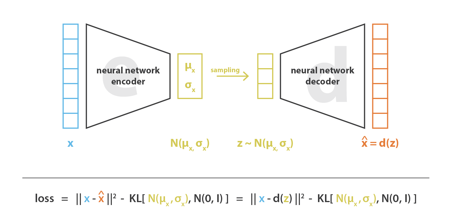
  • Variational Autoencoder (VAE) is an unsupervised latent variable model that learns a deep representation from high-dimensional data. The idea is to encode the input as a probability distribution rather than a point estimate as in vanilla auto-encoder. Then VAE uses a decoder to reconstruct the original input by using samples from that probability distribution.

    变分自动编码器(VAE)是一种无监督的潜在变量模型,可从高维数据中学习深度表示。 想法是将输入编码为概率分布,而不是像普通自动编码器那样将点估算为编码。 然后,VAE使用解码器通过使用来自该概率分布的样本来重建原始输入。

Image for post
Variational Autoencoder Architecture
可变自动编码器架构

Okay, it’s time to review the different auto-encoder based recommendation framework!

好的,现在该回顾一下基于自动编码器的不同推荐框架了!

1 —自动录制 (1 — AutoRec)

One of the earliest models that consider the collaborative filtering problem from an auto-encoder perspective is AutoRec from “Autoencoders Meet Collaborative Filtering” by Suvash Sedhain, Aditya Krishna Menon, Scott Sanner, and Lexing Xie.

其中,从自动编码器来角度来考虑协同过滤问题最早的车型是由“AutoRec 自动编码相约协同过滤 ”的Suvash Sedhain,阿迪亚梅农,斯科特·塞纳和乐星谢。

In the paper’s setting, there are m users, n items, and a partially filled user-item interaction/rating matrix R with dimension m x n. Each user u can be represented by a partially filled vector rᵤ and each item i can be represented by a partially filled vector rᵢ. AutoRec directly takes user rating vectors rᵤ or item rating rᵢ as input data and obtains the reconstructed rating at the output layer. There are two variants of AutoRec depending on two types of inputs: item-based AutoRec (I-AutoRec) and user-based AutoRec (U-AutoRec). Both of them have the same structure.

在论文的设置中,有m个用户,n个项目和一个维度为mx n的部分填充的用户-项目交互/评分矩阵R。 每个用户u可以由部分填充的矢量r 1表示,每个项目i可以由部分填充的矢量r 1表示。 AutoRec直接将用户评级向量rᵤ或项目评级rᵢ作为输入数据,并在输出层获得重建的评级。 根据两种输入类型,有两种AutoRec变体:基于项目的AutoRec( I-AutoRec )和基于用户的AutoRec( U-AutoRec )。 它们都具有相同的结构。

Image for post
Suvesh Sedhain et al. — AutoRec: Autoencoders Meet Collaborative Filtering ( https://dl.acm.org/doi/10.1145/2740908.2742726 )
Suvesh Sedhain等。 — AutoRec:自动编码器满足协同过滤( https://dl.acm.org/doi/10.1145/2740908.2742726 )

Figure 1 from the paper illustrates the structure of I-AutoRec. The shaded nodes correspond to observed ratings, and the solid connections correspond to weights that are updated for the input rᵢ.

本文的图1说明了I-AutoRec的结构。 阴影节点对应于观察到的额定值,而实心连接对应于针对输入rᵢ更新的权重。

Given the input rᵢ, the reconstruction is:

给定输入rᵢ,重建为:

Image for post
Equation 6
方程式6

where f and g are the activation functions, and the parameter Theta includes W, V, mu, and b.

其中f和g是激活函数,参数Theta包括W,V,mu和b。

AutoRec uses only the vanilla auto-encoder structure. The objective function of the model is similar to the loss function of auto-encoder:

AutoRec仅使用香草自动编码器结构 。 该模型的目标函数类似于自动编码器的损失函数:

Image for post
Equation 7
方程式7

This function can be optimized by resilient propagation (converges faster and produces comparable results) or L-BFGS (Limited-memory Broyden Fletcher Goldfarb Shanno algorithm).

可以通过弹性传播(收敛更快并产生可比较的结果)或L-BFGS(有限内存的Broyden Fletcher Goldfarb Shanno算法)来优化此功能。

Here are some important things about AutoRec:

这是有关AutoRec的一些重要事项:

  • I-AutoRec generally performs better than U-AutoRec. This is because the average number of ratings for each item is much more than the average number of ratings given by each user.

    I-AutoRec通常比U-AutoRec表现更好。 这是因为每个项目的平均评分数量远大于每个用户给出的平均评分数量。
  • Different combinations of activation functions affect the performance of AutoRec considerably.

    激活功能的不同组合会极大影响AutoRec的性能。
  • Increasing the number of hidden neurons or the number of layers improves model performance. This makes sense as expanding the dimensionality of the hidden layer allows AutoRec to have more capacity to simulate the input features.

    增加隐藏神经元的数量或层数可以提高模型性能。 这是有道理的,因为扩展隐藏层的尺寸可以使AutoRec具有更多的能力来模拟输入要素。
  • Adding more layers to formulate a deep network can lead to slight improvement.

    添加更多层以构成深层网络可导致轻微改善。

The TensorFlow code of the AutoRec model class is given below for illustration purpose:

下面出于示例目的给出了AutoRec模型类的TensorFlow代码:

For my TensorFlow implementation, I trained AutoRec architecture with a hidden layer of 500 units activated by a sigmoid non-linear function. Other hyper-parameters include a learning rate of 0.001, a batch size of 512, the Adam optimizer, and a lambda regularizer of 1.

对于我的TensorFlow实施 ,我训练了AutoRec体系结构,并通过S型非线性函数激活了500个隐藏单元的隐藏层。 其他超参数包括0.001的学习率,512的批量大小,Adam优化器和1的lambda正则化器。

2 — DeepRec (2 — DeepRec)

DeepRec is a model created by Oleisii Kuchaiev and Boris Ginsburg from NVIDIA, as seen in “Training Deep Autoencoders for Collaborative Filtering.” The model is inspired by the AutoRec model described above, with several important distinctions:

DeepRec是由NVIDIA的Oleisii Kuchaiev和Boris Ginsburg创建的模型,如“ 培训深度自动编码器以进行协作过滤 ”中所示。 该模型受上述AutoRec模型的启发,具有几个重要区别:

  • The network is much deeper.

    网络更深。
  • The model uses “scaled exponential linear units” (SELUs).

    该模型使用“比例指数线性单位”(SELU)。
  • The dropout rate is high.

    辍学率很高。
  • The authors use iterative output re-feeding during training.

    作者在训练过程中使用了迭代输出。
Image for post
Oleisii Kuchaiev and Boris Ginsburg — Training Deep Autoencoders for Collaborative Filtering ( Oleisii Kuchaiev和Boris Ginsburg —培训用于协作过滤的深度自动编码器( https://arxiv.org/abs/1708.01715https://arxiv.org/abs/1708.01715 ) )

2.1 —模型 (2.1 — Model)

The figure above depicts a typical 4-layer autoencoder network. The encoder has 2 layers e_1 and e_2, while the decoder has 2 layers d_1 and d_2. They are fused together on the representation z. The layers are represented as f(W * x + b), where f is some non-linear activation function. If the range of the activation function is smaller than that of the data, the last layer of the decoder should be kept linear. The authors found it to be very important for activation function f in hidden layers to contain a non-zero negative part, and use SELU units in most of their experiments.

上图描述了典型的4层自动编码器网络。 编码器具有2个层e_1和e_2,而解码器具有2个层d_1和d_2。 它们在表示z上融合在一起。 这些层表示为f(W * x + b),其中f是一些非线性激活函数。 如果激活函数的范围小于数据的范围,则解码器的最后一层应保持线性。 作者发现对于隐藏层中的激活函数f包含一个非零的负数部分并在他们的大多数实验中使用SELU单元非常重要。

2.2 —损失函数 (2.2 — Loss Function)

Since it doesn’t make sense to predict zeros in user’s representation vector x, the authors optimize the Masked Mean Squared Error loss:

由于预测用户表示向量x中的零没有意义,因此作者优化了Masked Mean Squareed Error Loss:

Image for post
Equation 8
方程式8

where r_i is the actual rating, y_i is the reconstructed rating, and m_i is a mask function such that m_i = 1 if r_i is not 0 else m_i = 0.

其中r_i是实际等级,y_i是重构等级,m_i是掩码函数,如果r_i不为0,则m_i = 1,否则m_i = 0。

2.3 — Dense Re-feeding

2.3 —重喂

During forward pass and inference pass, the model takes a user represented by his vector of ratings from the training set x. Note that x is very sparse, while the output of the decoder f(x) is dense and contains rating predictions for all items in the corpus. Thus, to explicitly enforce fixed-point constraint and perform dense training updates, the authors augment every optimization iteration with an iterative dense re-feeding step as follows:

在正向传递和推理传递期间,模型会采用用户来自训练集x的评分矢量表示的用户。 请注意,x非常稀疏,而解码器f(x)的输出很密集,并且包含了语料库中所有项目的评分预测。 因此,为了显式地执行定点约束并执行密集训练更新,作者使用迭代密集重新馈送步骤来增强每个优化迭代,如下所示:

  1. During the initial forward pass, given sparse input x, the model computes the dense output f(x) and the MMSE loss using equation 8.

    在初始正向通过期间,给定稀疏输入x,模型使用公式8计算密集输出f(x)和MMSE损耗。
  2. During the initial backward pass, the model computes the gradients and updates the weights accordingly.

    在初始后退过程中,模型将计算梯度并相应地更新权重。
  3. During the second forward pass, the model treats f(x) as a new data point and thus computes f(f(x)). Both f(x) and f(f(x)) become dense. The MMSE loss now has all m as non-zeros.

    在第二次向前通过期间,模型将f(x)视为新的数据点,从而计算f(f(x))。 f(x)和f(f(x))都变得密集。 MMSE损失现在将所有m都设为非零。
  4. During the second backward pass, the model again computes the gradients and updates the weights accordingly.

    在第二次向后遍历期间,模型再次计算梯度并相应地更新权重。

The TensorFlow code of the DeepRec model definition is given below for illustration purpose:

下面给出DeepRec模型定义的TensorFlow代码以进行说明:

For my TensorFlow implementation, I trained DeepRec with the following architecture: [n, 512, 512, 1024, 512, 512, n]. So n is the number of ratings that the user has given, the encoder has 3 layers of size (512, 512, 1034), the bottleneck layer has size 1024, and the decoder has 3 layers of size (512, 512, n). I trained the model using stochastic gradient descent with a momentum of 0.9, a learning rate of 0.001, a batch size of 512, and a dropout rate of 0.8. Parameters are initialized via the Xavier initialization scheme.

对于TensorFlow实施 ,我使用以下架构训练了DeepRec:[n,512,512,1024,512,512,n]。 所以n是用户给出的等级数,编码器的大小为3层(512、512、1034),瓶颈层的大小为1024,解码器的大小为3层(512、512,n) 。 我使用动量为0.9,学习率为0.001,批量为512,辍学率为0.8的随机梯度下降训练模型。 通过Xavier初始化方案初始化参数。

3 —协同降噪自动编码器 (3 — Collaborative Denoising Auto-encoder)

“Collaborative Denoising Autoencoders for Top-N Recommender Systems” by Yao Wu, Christopher DuBois, Alice Zheng, and Martin Ester is a neural network with one hidden layer. Compared to AutoRec and DeepRec, CDAE has the following differences:

吴耀,Christopher DuBois,Alice Zheng和Martin Ester 撰写的“用于Top-N推荐系统的协作降噪自动编码器 ”是一个具有一层隐藏层的神经网络。 与AutoRec和DeepRec相比, CDAE具有以下差异:

  • The input of CDAE is not user-item ratings, but partially observed implicit feedback r (user’s item preference). If a user likes a movie, the corresponding entry value is 1, otherwise 0.

    CDAE的输入不是用户项目评分,而是部分观察到的隐式反馈r(用户项目偏好)。 如果用户喜欢电影,则相应的输入值为1,否则为0。
  • Unlike the previous two models that are used for rating prediction, CDAE is principally used for ranking prediction (also called Top-N preference recommendations).

    与用于评级预测的前两个模型不同,CDAE主要用于排名预测(也称为Top-N偏好建议)。
Image for post
Yao Wu et al. — Collaborative Denoising Autoencoders For Top-N Recommender Systems ( https://dl.acm.org/doi/10.1145/2835776.2835837 )
姚武等。 —用于Top-N推荐系统的协作降噪自动编码器( https://dl.acm.org/doi/10.1145/2835776.2835837 )

3.1 —模型 (3.1 — Model)

The figure above shows a sample structure of CDAE, which consists of 3 layers: the input, the hidden, and the output.

上图显示了CDAE的示例结构,该结构由3层组成:输入,隐藏和输出。

  • There are a total of I + 1 nodes in the input layer. The first I nodes represent user preferences, and each node of these I nodes corresponds to an item. The last node is a user-specific node denoted by the red node in the figure above, which means different users have different nodes and associated weights.

    输入层中总共有I +1个节点。 前I个节点代表用户首选项,这些I节点中的每个节点都对应一个项目。 最后一个节点是特定于用户的节点,在上图中用红色节点表示,这意味着不同的用户具有不同的节点和关联的权重。
  • Here yᵤ is the I-dimensional feedback vector of user u on all the items in I. yᵤ is a sparse binary vector that only has non-zero values: yᵤᵢ = 1 if i has been rated by user u and yᵤᵢ = 0 otherwise.

    此处yᵤ是用户u在I中所有项目上的I维反馈矢量。yᵤ是稀疏的二进制矢量,仅具有非零值:如果i被用户u评分,则yᵤᵢ= 1,否则y = 0。
  • There are K (<< I) + 1 nodes in the hidden layer. The blue K nodes are fully connected to the nodes of the input layer. The pink additional node in the hidden layer captures the bias effects.

    隐藏层中有K(<< I)+ 1个节点。 蓝色的K节点完全连接到输入层的节点。 隐藏层中的粉红色附加节点捕获了偏见效果。
  • In the output layer, there are I nodes which are the reconstructed output of the input yᵤ. They are fully connected to the nodes in the hidden layer.

    在输出层中,有I个节点,它们是输入yᵤ的重构输出。 它们完全连接到隐藏层中的节点。

The corrupted input r_corr of CDAE is drawn from a conditional Gaussian distribution p(r_corr | r). The reconstruction of r_corr is formulated as follows:

CDAE的损坏输入r_corr从条件高斯分布p(r_corr | r)中提取r_corr的重建公式如下:

Image for post
Equation 9
式9

where W₁ is the weight matrix corresponding to the encoder (going from the input layer to the hidden layer), W₂ is the weight matrix corresponding to the decoder (going from the hidden layer to the output layer). Vᵤ is the weight matrix for the red user node, while both b₁ and b₂ are the bias vectors.

其中W 1是对应于编码器的权重矩阵(从输入层到隐藏层),W 2是对应于解码器的权重矩阵(从隐藏层到输出层)。 V 1是红色用户节点的权重矩阵,而b 1和b 2都是偏差矢量。

3.2 —损失函数 (3.2 — Loss Function)

The parameters of CDAE are learned by minimizing the average reconstruction error as follows:

通过使平均重构误差最小化来学习CDAE的参数,如下所示:

Image for post
Equation 10
式10

The loss function L(r_corr, h(r_corr)) in the equation above can be square loss or logistic loss. CDAE uses the square L2 norm to control the model complexity. It also (1) applies stochastic gradient descent to learn the model’s parameters and (2) adopts AdaGrad to automatically adapt the training step size during the learning procedure.

上式中的损失函数L (r_corr,h(r_corr))可以是平方损失或逻辑损失。 CDAE使用平方L2范数来控制模型的复杂性。 它还(1)应用随机梯度下降来学习模型的参数,(2)采用AdaGrad在学习过程中自动调整训练步长。

The authors also propose a negative sampling technique to extract a small subset from items that user did not interact with for reducing the time complexity substantially without degrading the ranking quality. At inference time, CDAE takes a user’s existing preference set (without corruption) as input and recommends the items with the largest prediction values on the output layer to that user.

作者还提出了一种负采样技术,可以从用户未与之交互的项目中提取一小部分子集,从而在不降低排名质量的前提下,大幅降低了时间复杂度。 在推断时,CDAE将用户的现有首选项集(无损坏)作为输入,并向该用户推荐输出层上具有最大预测值的项目。

The PyTorch code of the CDAE architecture class is given below for illustration purpose:

出于说明目的,下面给出了CDAE体系结构类的PyTorch代码:

For my PyTorch implementation, I used a CDAE architecture with a hidden layer of 50 units. I trained the model using stochastic gradient descent with a learning rate of 0.01, a batch size of 512, and a corruption ratio of 0.5.

对于我的PyTorch实施 ,我使用了带有50个隐藏层的CDAE体系结构。 我使用随机梯度下降训练模型,学习率为0.01,批处理大小为512,损坏比为0.5。

4 —多项式变分自动编码器 (4 — Multinomial Variational Auto-encoder)

One of the most influential papers in this discussion is “Variational Autoencoders for Collaborative Filtering” by Dawen Liang, Rahul Krishnan, Matthew Hoffman, and Tony Jebara from Netflix. It proposes a variant of VAE for recommendation with implicit data. In particular, the authors introduced a principled Bayesian inference approach to estimate model parameters and show favorable results than commonly used likelihood functions.

讨论中最具影响力的论文之一是Netflix的Dawen Liang,Rahul Krishnan,Matthew Hoffman和Tony Jebara撰写的“ 协作过滤的变体自动编码器 ”。 它提出了一种VAE的变体,用于带有隐式数据的推荐。 特别是,作者引入了一种有原则的贝叶斯推理方法来估计模型参数并显示出比常用似然函数更好的结果。

The paper uses U to index all users and I to index all items. The user-by-item interaction matrix is called X (with dimension U x I). The lower case xᵤ is a bag-of-words vector with the number of clicks for each item from user u. For implicit feedback, this matrix is binarized to have only 0s and 1s.

本文使用U索引所有用户,使用I索引所有项目。 用户与项目的交互矩阵称为X(尺寸为U x I)。 小写的xᵤ是一个词袋向量,其中包含用户u对每个项目的点击次数。 对于隐式反馈,此矩阵被二值化为只有0和1。

4.1 —模型 (4.1 — Model)

Image for post
Equation 11
式11

The generative process of the model is seen in equation 11 and broken down as follows:

该模型的生成过程如公式11所示,分解如下:

  • For each user u, the model samples a K-dimensional latent representation zᵤ from a standard Gaussian prior.

    对于每个用户u,模型从标准高斯先验样本中抽取K维潜在表示zᵤ。
  • Then it transforms zᵤ via a non-linear function f_θ to produce a probability distribution over I items π(zᵤ).

    然后,它通过非线性函数f_θ变换zᵤ,以在I个项π(zᵤ)上产生概率分布。
  • f_θ is a multi-layer perceptron with parameters θ and a softmax activation function.

    f_θ是具有参数θ和softmax激活函数的多层感知器。
  • Given the total number of clicks from user u, the bag-of-words vector xᵤ is sampled from a multinomial distribution with probability π(zᵤ).

    给定用户u的总点击次数,从多项式分布中以概率π(zᵤ)采样词袋矢量xᵤ。

The log-likelihood for user u (conditioned on the latent representation) is:

用户u的对数似然(取决于潜在表示):

Image for post
Equation 12
式12

The authors believe that the multinomial distribution is suitable for this collaborative filtering problem. Specifically, the likelihood of the interaction matrix in equation 11 rewards the model for putting probability mass on the non-zero entries in xᵤ. However, considering that π(zᵤ) must sum to 1, the items must compete for a limited budget of probability mass. Therefore, the model should instead assign more probability mass to items that are more likely to be clicked, making it suitable to achieve a solid performance in the top-N ranking evaluation metric of recommendation systems.

作者认为, 多项式分布适用于此协作过滤问题。 具体地,等式11中的相互作用矩阵的似然性奖励了将概率质量置于x 1中的非零项上的模型。 但是,考虑到π(zᵤ)必须等于1,因此这些项目必须竞争概率质量有限的预算。 因此,该模型应改为为更有可能被点击的项目分配更多的概率质量,使其适合于在推荐系统的前N名评估指标中获得可靠的表现。

4.2 —变分推理 (4.2 — Variational Inference)

In order to train the generative model in equation 11, the authors estimate θ by approximating the intractable posterior distribution p(zᵤ | xᵤ) via variational inference. This method approximates the true intractable posterior with a simpler variational distribution q(zᵤ) — which is a fully diagonal Gaussian distribution. The objective of variational inference is to optimize the free variational parameters {μᵤ, σᵤ²} so that the Kullback-Leiber divergence KL(q(zᵤ) || p(zᵤ | xᵤ)) is minimized.

为了训练等式11中的生成模型,作者通过变分推断通过近似难处理的后验分布p(zᵤ|xᵤ)来估计θ。 该方法用更简单的变化分布q(zᵤ)逼近了真正的难治性后验,后者是完全对角的高斯分布。 变分推论的目的是优化自由变分参数{μᵤ,σᵤ²},以使Kullback-Leiber发散KL(q(zᵤ)|| p(zᵤ|xᵤ))最小。

The issue with variational inference is that the number of parameters to optimize {μᵤ, σᵤ²} grows with the number of users and items in the dataset. VAE helps solve this issue by replacing the individual variational parameters with a data-dependent function:

变异推理的问题在于,优化{μᵤ,σᵤ²}的参数数量随数据集中用户和项目数量的增加而增加。 VAE通过使用依赖于数据的函数替换各个变分参数来帮助解决此问题:

Image for post
Equation 13
式13

This function is parameterized by ϕ — in which both μ_{ϕ} (xᵤ) and σ_{ϕ} (xᵤ) are vectors with K dimensions. The variational distribution is then set as follows:

此函数由ϕ参数化,其中μ_{ϕ}(xᵤ)和σ_{ϕ}(xᵤ)均为K维向量。 然后按照以下方式设置变化分布:

Image for post
Equation 14
式14

Using the input xᵤ, the inference model returns the corresponding variational parameters of variational distribution q_{ϕ} (zᵤ|xᵤ). When being optimized, this variational distribution approximates the intractable posterior p_{ϕ} (zᵤ | xᵤ).

使用输入xᵤ,推理模型返回相应的变化量分布q_ {ϕ}(zᵤ|xᵤ)的变化参数。 当优化时,该变化分布近似于难处理的后验p_ {ϕ}(zᵤ|xᵤ)。

Image for post
Variational Gradient ( 梯度变化( https://matsen.fredhutch.org/general/2019/08/24/vbpi.htmlhttps://matsen.fredhutch.org/general/2019/08/24/vbpi.html ) )

To learn latent-variable models with variational inference, the standard approach is to lower-bound the log marginal likelihood of the data. The objective function to maximize for user u now becomes:

要学习具有变分推断的潜变量模型,标准方法是降低数据的对数边际可能性。 现在,为用户u最大化的目标函数变为:

Image for post
Equation 15
式15

Another term to call this objective is evidence lower bound (ELBO). Intuitively, we should be able to obtain an estimate of ELBO by sampling zᵤ ∼ q_ϕ and optimizing it with a stochastic gradient ascent. However, we cannot differentiate ELBO to get the gradients with respect to ϕ. The reparametrization trick comes in handy here:

称为该目标的另一个术语是证据下界(ELBO)。 凭直觉,我们应该能够通过采样zᵤ〜q_ϕ并用随机梯度上升对其进行优化来获得ELBO的估计。 但是,我们无法区分ELBO来获得相对于ϕ的梯度。 重新参数化技巧在这里派上用场:

Image for post
Equation 16
式16

Essentially, we isolate the stochasticity in the sampling process, and thus the gradient with respect to ϕ can be back-propagated through the sampled zᵤ.

本质上,我们在采样过程中隔离了随机性,因此,相对于的梯度可以通过采样的z with反向传播。

From a different perspective, the first term of equation 15 can be interpreted as reconstruction error and the second term of equation 15 can be interpreted as regularization. The authors, therefore, extend equation 15 with an additional parameter β to control the strength of regularization:

从不同的角度来看,方程式15的第一项可以解释为重构误差 ,方程式15的第二项可以解释为正则化 。 因此,作者用附加参数β扩展了等式15,以控制正则化的强度:

Image for post
Equation 17
式17

This parameter β engages a tradeoff between how well the model fits the data and how close the approximate posterior stays to the prior during learning. The authors tune β via KL annealing, a common heuristic used for training VAEs when there is concern that the model is being under-utilized.

该参数β在模型拟合数据的程度与学习中近似后验与前验之间的距离之间进行折衷。 作者通过KL退火 (一种用于训练VAE的常见启发式方法)对β进行调整,当担心模型未得到充分利用时。

4.3 —预测 (4.3 — Prediction)

Given a user’s click history x, the model ranks all items based on the un-normalized predicted multinomial probability f_ϕ (z). The latent representation z for x is simply the mean of the variational distribution z = μ_ϕ (x).

给定用户的点击历史记录x,该模型会根据未归一化的预测多项式概率f_(z)对所有项目进行排名。 x的潜在表示z只是变化分布z =μ_(x)的平均值。

Image for post
Dawen Liang et al. — Variational Autoencoders for Collaborative Filtering ( https://arxiv.org/abs/1802.05814 )
梁大文等。 —用于协作过滤的变体自动编码器( https://arxiv.org/abs/1802.05814 )

Figure 2 from the paper provides a unified view of different variants of autoencoders.

本文的图2提供了自动编码器不同变体的统一视图。

  • 2a is the vanilla auto-encoder architecture, as seen in AutoRec and DeepRec.

    2a是香草自动编码器架构,如AutoRec和DeepRec中所示。
  • 2b is the denoising auto-encoder architecture, as seen in CDAE. Here ϵ is a noise injected to the input layer.

    如图2b所示,是CDAE中的降噪自动编码器架构。 ϵ是注入到输入层的噪声。
  • 2c is the variational auto-encoder architecture under MultVAE, which uses an inference model parametrized by ϕ to produce the mean and variance of the approximating variational distribution, as explained in detail above.

    2c是MultVAE下的变分自动编码器体系结构,它使用参数化为ϕ的推理模型来生成近似变分分布的均值和方差,如上所详细解释。

The PyTorch code of the MultVAE architecture class is given below for illustration purpose:

下面给出了MultVAE体系结构类的PyTorch代码以进行说明:

For my PyTorch implementation, I keep the architecture for the generative model f and the inference model g symmetrical and use an MLP with 1 hidden layer. The dimension of the latent representation K is set to 200 and of other hidden layers is set to 600. The overall architecture for a MultVAE now becomes [I -> 600 -> 200 -> 600 -> I], where I is the total number of items. Other model details include tanH activation function, dropout rate with probability 0.5, Adam optimizer, batch size of 512, and learning rate of 0.01.

对于我的PyTorch实施 ,我使生成模型f和推理模型g的体系结构保持对称,并使用具有1个隐藏层的MLP。 潜在表示K的尺寸设置为200,其他隐藏层的尺寸设置为600。MultVAE的总体体系结构现在变为[I-> 600-> 200-> 600-> I],其中I是总数项目数。 其他模型详细信息包括tanH激活函数,概率为0.5的辍学率,Adam优化器,批处理大小为512,学习率为0.01。

5 —顺序变分自动编码器 (5 — Sequential Variational Auto-encoder)

In “Sequential Variational Auto-encoders for Collaborative Filtering,” Noveen Sachdeva, Giuseppe Manco, Ettore Ritacco, and Vikram Pudi propose an extension of MultVAE by exploring the rich information present in the past preference history. They introduce a recurrent version of MultVAE, where instead of passing a subset of the whole history regardless of temporal dependencies, they pass the consumption sequence subset through a recurrent neural network. They show that handling temporal information is crucial for improving the accuracy of VAE.

Noveen Sachdeva,Giuseppe Manco,Ettore Ritacco和Vikram Pudi在“ 用于协作过滤的顺序变分自动编码器 ”中,通过探索过去的优先选择历史中存在的丰富信息,提出了MultVAE的扩展。 他们引入了MultVAE的循环版本 ,而不是传递整个历史的子集而不考虑时间依赖性,而是通过循环神经网络传递了消费序列子集。 他们表明, 处理时间信息对于提高VAE的准确性至关重要。

5.1 —设置 (5.1 — Setting)

The problem setting is exactly similar to that of the MultVAE paper: U is a set of users, I is a set of items, and X is the user-item preference matrix with dimension U x I. The principal difference is that SVAE considers precedence and temporal relationships within the matrix X.

问题设置与MultVAE论文的设置完全相似:U是一组用户,I是一组项目,X是维度为U x I的用户项偏好矩阵。主要区别在于SVAE考虑了优先级矩阵X中的时间和时间关系。

  • X induces a natural ordering relationship between items: i <ᵤ j has the meaning that x_{u, i} > x_{u, j} in the rating matrix.

    X引起项目之间的自然排序关系:i <ᵤj的含义是,评级矩阵中的x_ {u,i}> x_ {u,j}。
  • They assume the existence of timing information T, where the term t_{u,i} represents the time when i was chosen by u. Then i <ᵤ j denotes that t_{u, i} > t_{u, j}.

    他们假设存在定时信息T,其中术语t_ {u,i}表示u选择i的时间。 然后,i <ᵤj表示t_ {u,i}> t_ {u,j}。
  • They also introduce a temporal mark in the elements of xᵤ: x_{u(t)} represents the t-th item in Iᵤ in the sorting induced by <ᵤ, whereas x_{u(1:t)} represents the sequence from x_{u(1)} to x_{u(t)}.

    他们还在xᵤ的元素中引入了一个时间标记:x_ {u(t)}表示<ᵤ诱导的排序中Iᵤ中的第t个项,而x_ {u(1:t)}表示来自x_的序列{u(1)}至x_ {u(t)}。
Image for post
Noveen Sachdeva et al. — Sequential Variational Autoencoders for Collaborative Filtering ( https://arxiv.org/abs/1811.09975 )
Noveen Sachdeva等。 —用于协同过滤的顺序变分自动编码器( https://arxiv.org/abs/1811.09975 )

5.2 —模型 (5.2 — Model)

The figure above from the paper shows the architectural difference between MultVAE, SVAE, and another model called RVAE (which I won’t discuss here). Looking at the SVAE architecture, I can observe the recurrent relationship occurring in the layer upon which z_{u(t)} depends. The basic idea behind SVAE is that latent variable modeling should be able to express temporal dynamics and hence causalities and dependencies among preferences in a user’s history.

论文的上图显示了MultVAE,SVAE和另一个称为RVAE的模型(在此不再讨论)之间的体系结构差异。 查看SVAE体系结构,我可以观察到z_ {u(t)}所依赖的层中发生的递归关系。 SVAE的基本思想是, 潜在变量建模应该能够表达时间动态 ,从而 能够表达 用户历史记录中偏好之间的因果关系和依存关系

Let’s review the math. Within this SVAE framework, the authors model temporal dependencies by conditioning each event to the previous events. Given a sequence x_{(1: T}, then its probability is:

让我们回顾一下数学。 在此SVAE框架内,作者通过将每个事件调整为先前的事件来对时间依赖性进行建模。 给定序列x _ {(1:T},则其概率为:

Image for post
Equation 18
式18

This probability represents a recurrent relationship between x_{(t+1} and x_{(1:t)}. Thus, the model can handle each timestep separately.

该概率表示x _ {(t + 1}与x _ {(1:t)}之间的递归关系,因此,该模型可以分别处理每个时间步长。

Recall the generative process in equation 11, we can add a timestamp t as seen below:

回想一下方程11中的生成过程,我们可以添加一个时间戳t,如下所示:

Image for post
Equation 19
式19

Equation 19 results in the joint likelihood:

公式19得出联合可能性:

Image for post
Equation 20
式20

The posterior likelihood in equation 20 can be approximated with a factorized proposal distribution:

方程20中的后验似然可以通过分解后的提案分布进行近似计算:

Image for post
Equation 21
式21

where the right-term side is a Gaussian distribution whose parameters μ and σ depend upon the current history x_{u(1:t-1)}, by means of a recurrent layer h_t:

其中右边项是高斯分布,其参数μ和σ通过循环层h_t取决于当前历史x_ {u(1:t-1)}:

Image for post
Equation 22
式22

Finally, the loss function that SVAE optimized is:

最后,SVAE优化的损失函数为:

Image for post
Equation 23
式23

5.3 —预测 (5.3 — Prediction)

In this SVAE model, the proposal distribution introduces a dependency of the latent variable from a recurrent layer, which allows us to recover the information from the previous history. Given a user history x_{u(1:t-1)}, we can use equation 22 and set z = μ_{λ} (t), upon which we can devise the probability for the x_{u(t)} by means of π(z).

在此SVAE模型中,投标分布引入了来自递归层的潜在变量的依赖性,这使我们能够从先前的历史中恢复信息 。 给定用户历史记录x_ {u(1:t-1)},我们可以使用公式22并设置z =μ_{λ}(t),然后根据该公式设计x_ {u(t)}的概率π(z)的均值。

The PyTorch code of the SVAE architecture class is given below for illustration purpose:

出于说明目的,以下给出了SVAE体系结构类的PyTorch代码:

Another unique property of this paper is the way the evaluation protocol works. The authors partitioned users into training, validation, and test set; and then trained the model using the full histories of the users in the training set. During the evaluation, for each user in the validation/test set, they split the time-sorted user history into two parts, fold-in and fold-out split.

本文的另一个独特属性是评估协议的工作方式。 作者将用户划分为训练,验证和测试集。 然后使用训练集中用户的全部历史训练模型。 在评估过程中,对于验证/测试集中的每个用户,他们将按时间排序的用户历史记录分为两部分,即折叠折叠

  • The fold-in split learns the necessary representations and recommends items.

    折入式拆分学习必要的表示形式并推荐商品。

  • These items are then evaluated with the fold-out split of the user history using metrics such as Precision, Recall, and Normalized Discounted Cumulative Gain.

    然后,使用“精度”,“召回率”和“标准化折扣累积收益”等指标,通过用户历史记录的展开式拆分来评估这些项目。

For my PyTorch implementation, I follow the same code provided by the authors.

对于我的PyTorch实现 ,我遵循作者提供的相同代码。

  • The SVAE architecture includes an embedding layer of size 256, a recurrent layer (Gated Recurrent Unit) with 200 cells, and two encoding layers (of size 150 and 64) and finally two decoding layers (of size 64 and 150).

    SVAE体系结构包括大小为256的嵌入层,具有200个单元的循环层(门控循环单元),两个编码层(大小为150和64)以及最后两个解码层(大小为64和150)。
  • The number K of latent factors for the VAE is set to be 64.

    VAE的潜在因子数K设置为64。
  • The model is optimized with Adam and weight decay is set to be 0.01.

    该模型使用Adam优化,权重衰减设置为0.01。

6 —尴尬的浅层自动编码器 (6 — Embarrassingly Shallow Auto-encoders)

Harald Steck’s “Embarrassingly Shallow Autoencoders for Sparse Data” is a fascinating one that I want to bring into this discussion. The motivation here is that, according to his literature review, deep models with a large number of hidden layers typically do not obtain a notable improvement in ranking accuracy in collaborative filtering, compared to ‘deep’ models with only one, two, or three hidden layers. This is a stark contrast to other areas like NLP or computer vision.

Harald Steck的“ 稀疏数据的令人尴尬的浅自动编码器 ”是我想引入这个讨论的一个有趣的例子。 根据他的文献综述, 这样做的动机是, 与只有一个,两个或三个隐藏的“深层”模型相比 ,具有大量隐藏层的深层模型 在协作过滤中的排名准确性 通常 不会 获得显着提高。层。 与NLP或计算机视觉等其他领域形成鲜明对比。

Image for post
Harald Steck — Embarrassingly Shallow Autoencoders for Sparse Data ( Harald Steck-稀疏数据的尴尬的浅自动编码器( https://arxiv.org/abs/1905.03375https://arxiv.org/abs/1905.03375 ) )

6.1 —模型 (6.1 — Model)

Embarrassingly Shallow Auto-encoders (ESAE) is a linear model without a hidden layer. The (binary) input vector X vector indicates which items a user has interacted with, and ESAE’s objective is to predict the best items to recommend to that user in the output layer (as seen in the figure above). For implicit feedback, a value of 1 in X indicates that the user interacted with an item, while a value of 0 in X indicates that there is no observed interaction.

令人尴尬的浅层自动编码器 (ESAE)是没有隐藏层的线性模型。 (二进制)输入向量X向量指示用户与哪些项目进行了交互,并且ESAE的目标是预测在输出层中推荐给该用户的最佳项目(如上图所示)。 对于隐式反馈,X中的值为1表示用户与某个项目进行了交互,而X中的值为0表示没有观察到的交互。

The item-item weight matrix B represents the parameters of ESAE. Here, the self-similarity of an item in the input layer with itself in the output layer is omitted, so that ESAE can generalize effectively during the reconstruction step. Thus, the diagonal of this weight-matrix B is constrained to 0 (diag(B) = 0).

项目权重矩阵B代表ESAE的参数。 在此,省略了输入层中的项目与输出层中的项目之间的自相似性,因此ESAE可以在重建步骤中有效地进行泛化。 因此,该权重矩阵B的对角线被约束为0( diag(B)= 0 )。

For an item j and a user u, we want to predict S_{u, j}, where X_{u,.} refers to row u and B_{.,j} refers to column j:

对于项目j和用户u,我们要预测S_ {u,j},其中X_ {u ,.}表示行u,而B _ {。,j}表示列j:

Image for post
Equation 24
式24

6.2 —目标函数 (6.2 — Objective Function)

With respect to diag(B) = 0, ESAE has the following convex objective for learning the weights B:

关于diag(B)= 0, ESAE具有以下凸目标,用于学习权重B:

Image for post
Equation 25
式25

Here are important notes about this convex objective:

以下是有关此凸目标的重要说明:

  • ||.|| denotes the Frobenius norm. This squared loss between the data X and the predicted scores XB allows for a closed-form solution.

    ||。|| 表示Frobenius范数 。 数据X和预测分数XB之间的平方损失允许采用封闭形式的解决方案

  • The hyper-parameter λ is the L2-norm regularization of the weights B.

    超参数λ是权重B的L2-范数正则化。
  • The constraint of a zero diagonal helps avoid the trivial solution B = I where I is the identity matrix.

    对角线为零的约束有助于避免平凡解B = I,其中I是单位矩阵。

In the paper, Harald derived a closed-form solution from the training objective in equation 25. He argues that the traditional neighborhood-based collaborative filtering approaches are based on conceptually incorrect item-item similarity matrices, while the ESAE framework utilizes principled neighborhood models. I won’t go over the math derivation here, but you should take a look at section 3.1 from the paper for the detail.

在本文中,Harald从等式25中的训练目标中得出了一种封闭形式的解决方案。他认为,传统的基于邻域的协作过滤方法基于概念上不正确的项-项相似度矩阵,而ESAE框架则采用了原则性的邻域模型。 我不会在这里讨论数学推导,但是您应该看一下论文中的3.1节以获取详细信息。

Notably, ESAE’s similarity matrix is based on the inverse of the given data matrix. As a result, the learned weights can also be negative and thus the model can learn the dissimilarities between items (besides the similarities). This proves to be essential to obtain good ranking accuracy. Furthermore, the data sparsity problem (there possibly is only a small amount of data available for each user) does not affect the uncertainty in estimating weight matrix B if the number of users in the data matrix X is sufficiently large.

值得注意的是,ESAE的相似性矩阵是基于给定数据矩阵的矩阵。 结果,学习的权重也可以是负的,因此模型可以学习项目之间的差异 (除了相似性之外)。 事实证明,这对于获得良好的排名准确性至关重要。 此外,如果数据矩阵X中的用户数足够大,则数据稀疏性问题( 每个用户可能只有少量数据可用)不会影响估计权重矩阵B的不确定性。

6.3 —算法 (6.3 — Algorithm)

The Python code of the learning algorithm is given above. The training requires only the item-item matrix G = X^T * X as input, instead of the user-item matrix X. This is very efficient if the size of G is smaller than the size of X.

上面给出了学习算法的Python代码。 训练仅需要输入项目矩阵G = X ^ T * X,而不是用户项目矩阵X。如果G的大小小于X的大小,这将非常有效。

For my PyTorch implementation, I set the L2-Norm regularization hyper-parameter λ to be 1000, the learning rate to be 0.01, and the batch size to be 512.

对于我的PyTorch实施 ,我将L2-Norm正则化超参数λ设置为1000,学习率设置为0.01,批处理大小设置为512。

模型评估 (Model Evaluation)

You can check out all six autoencoder-based recommendation models that I built at this repository: https://github.com/khanhnamle1994/transfer-rec/tree/master/Autoencoders-Experiments.

您可以检出我在此存储库中构建的所有六个基于自动编码器的推荐模型: https : //github.com/khanhnamle1994/transfer-rec/tree/master/Autoencoders-Experiments

  • The dataset is MovieLens 1M, similar to the two previous experiments that I have done using Matrix Factorization and Multilayer Perceptron. The goal is to predict the ratings that a user will give to a movie, in which the ratings are between 1 to 5.

    数据集是MovieLens 1M ,类似于我之前使用矩阵分解多层感知器进行的两个实验。 目的是预测用户对电影的评分,其中评分介于1到5之间。

  • For the AutoRec and DeepRec models, the evaluation metric is Masked Root Mean Squared Error (RMSE) in a rating prediction (regression) setting.

    对于AutoRec和DeepRec模型,评估指标为等级预测(回归)设置中的掩盖均方根误差(RMSE)

  • For the CDAE, MultVAE, SVAE, and ESAE models, the evaluation metrics are Precision, Recall, and Normalized Discounted Cumulative Gain (NDCG) in a ranking prediction (classification) setting. As explained in the sections above, these models work with implicit feedback data, where ratings are binarized into 0 (less than equal to 3) and 1 (bigger than 3).

    对于CDAE,MultVAE,SVAE和ESAE模型,评估指标是在排名预测(分类)设置中的PrecisionRecallNormalized Discounted Cumulative Gain(NDCG) 。 如以上各节所述,这些模型适用于隐式反馈数据,其中评级被二进制化为0(小于等于3)和1(大于3)。

  • The results were captured in Comet ML. For those that are not familiar, it is a fantastic tool that keeps track of model experiments and logs all necessary metrics in a single dashboard.

    结果在彗星ML中捕获。 对于不熟悉的人来说,它是一个了不起的工具,可以跟踪模型实验并将所有必要的指标记录在一个仪表板上。

The result table is at the bottom of my repo’s README:

结果表位于我的回购自述文件的底部:

Image for post
Model Evaluation
模型评估

For rating prediction:

对于评分预测:

  • AutoRec performs better than DeepRec: lower RMSE and shorter runtime.

    AutoRec的性能优于DeepRec:更低的RMSE和更短的运行时间。
  • This is quite surprising, as DeepRec is a deeper architecture than AutoRec.

    这非常令人惊讶,因为DeepRec是比AutoRec更深的体系结构。

For ranking prediction:

对于排名预测:

  • The SVAE model clearly has the best result; however, it also takes an order of magnitude longer to train.

    SVAE模型显然具有最佳结果。 但是,训练也需要一个数量级以上的时间。
  • Between the remaining three models: CDAE has the highest Precision@100, ESAE has the highest Recall@100 and NDCG@100, and MultVAE has the shortest runtime.

    在其余三个模型之间:CDAE的Precision @ 100最高,ESAE的Recall @ 100和NDCG @ 100最高,MultVAE的运行时间最短。

结论 (Conclusion)

In this post, I have discussed the nuts and bolts of Auto-encoders and their use in collaborative filtering. I also walked through 6 different papers that use Auto-encoders for the recommendation framework: (1) AutoRec, (2) DeepRec, (3) Collaborative Denoising Auto-encoder, (4) Multinomial Variational Auto-encoder, (5) Sequential Variational Auto-encoder, and (6) Embarrassingly Shallow Auto-encoder.

In this post, I have discussed the nuts and bolts of Auto-encoders and their use in collaborative filtering. I also walked through 6 different papers that use Auto-encoders for the recommendation framework: (1) AutoRec, (2) DeepRec, (3) Collaborative Denoising Auto-encoder, (4) Multinomial Variational Auto-encoder, (5) Sequential Variational Auto-encoder, and (6) Embarrassingly Shallow Auto-encoder.

There are several emerging research directions that are happening in this area:

There are several emerging research directions that are happening in this area:

  • When facing different recommendation requirements, it is important to incorporate auxiliary information to help understand users and items to further improve the performance of recommendation. The capacity of auto-encoders to process heterogeneous data sources brings great opportunities in recommending diverse items with unstructured data such as text, images, audio, and video features.

    When facing different recommendation requirements, it is important to incorporate auxiliary information to help understand users and items to further improve the performance of recommendation. The capacity of auto-encoders to process heterogeneous data sources brings great opportunities in recommending diverse items with unstructured data such as text, images, audio, and video features.
  • Many effective unsupervised learning techniques based on auto-encoders have recently emerged: weighted auto-encoders, ladder variational auto-encoders, and discrete variational auto-encoders. Using these new auto-encoders variants will help improve the recommendation performance even further.

    Many effective unsupervised learning techniques based on auto-encoders have recently emerged: weighted auto-encoders, ladder variational auto-encoders, and discrete variational auto-encoders. Using these new auto-encoders variants will help improve the recommendation performance even further.
  • Besides collaborative filtering, one can integrate the auto-encoders paradigm with content-based filtering and knowledge-based recommendation methods. These are largely under-explored areas that have the potential for progress.

    Besides collaborative filtering, one can integrate the auto-encoders paradigm with content-based filtering and knowledge-based recommendation methods. These are largely under-explored areas that have the potential for progress.

Stay tuned for future blog posts of this series that explore different modeling architectures that have been made for collaborative filtering.

Stay tuned for future blog posts of this series that explore different modeling architectures that have been made for collaborative filtering.

If you would like to follow my work on Recommendation Systems, Deep Learning, and Data Science Journalism, you can check out my Medium and GitHub, as well as other projects at https://jameskle.com/. You can also tweet at me on Twitter, email me directly, or find me on LinkedIn. Sign up for my newsletter to receive my latest thoughts on machine learning in research and in the industry right at your inbox!

If you would like to follow my work on Recommendation Systems, Deep Learning, and Data Science Journalism, you can check out my Medium and GitHub , as well as other projects at https://jameskle.com/ . You can also tweet at me on Twitter , email me directly , or find me on LinkedIn . Sign up for my newsletter to receive my latest thoughts on machine learning in research and in the industry right at your inbox!

翻译自: https://towardsdatascience.com/recommendation-system-series-part-6-the-6-variants-of-autoencoders-for-collaborative-filtering-bd7b9eae2ec7

gan的几种变体

  • 1
    点赞
  • 6
    收藏
    觉得还不错? 一键收藏
  • 0
    评论

“相关推荐”对你有帮助么?

  • 非常没帮助
  • 没帮助
  • 一般
  • 有帮助
  • 非常有帮助
提交
评论
添加红包

请填写红包祝福语或标题

红包个数最小为10个

红包金额最低5元

当前余额3.43前往充值 >
需支付:10.00
成就一亿技术人!
领取后你会自动成为博主和红包主的粉丝 规则
hope_wisdom
发出的红包
实付
使用余额支付
点击重新获取
扫码支付
钱包余额 0

抵扣说明:

1.余额是钱包充值的虚拟货币,按照1:1的比例进行支付金额的抵扣。
2.余额无法直接购买下载,可以购买VIP、付费专栏及课程。

余额充值