绝缘子工作温度_在温度下工作

绝缘子工作温度

One of the hypotheses that the scientific community is working on is the option that the SARS-CoV-2 coronavirus is less transmissible in the presence of a warm and humid climate, a possibility that could reduce the incidence of COVID-19 disease as the spring progresses, the summer months get closer and it becomes warmer. For the time being, this is only a hypothesis, since although there are preliminary studies that point in that direction, there is still not enough scientific evidence to say that the virus survives worse in heat and that the pandemic could be attenuated by the arrival of higher temperatures or a more humid climate.

科学界正在研究的一种假设是，在温暖潮湿的气候下，SARS-CoV-2冠状病毒的传播可能性较小，这种可能性可能会降低SpringSpringCOVID-19疾病的发病率进展，夏季越来越近，天气变得越来越暖和。 暂时，这只是一个假设，因为尽管有朝着这个方向进行的初步研究，但仍然没有足够的科学证据表明该病毒在高温下生存较差，并且流行病可能会随着流感的到来而减弱。更高的温度或更潮湿的气候。

Some respiratory viruses, such as influenza, are known to spread more during the cold-climate months, and the other known coronavirus generally survives worse in higher temperatures and greater humidity than in colder or drier environments. There are some reasons for the seasonality of viruses in temperate regions, but the information is still lacking as to whether this theory can be applied to the new coronavirus.

已知某些呼吸道病毒(例如流行性感冒)在寒冷气候月份传播更多，而另一种冠状病毒通常在较高温度和较高湿度下的生存能力较寒冷或干燥的环境差。 温带地区病毒的季节性存在某些原因，但仍缺乏有关该理论是否可以应用于新冠状病毒的信息。

数据概述： (Data Overview :)

The rising average temperature of Earth’s climate system, called global warming, is driving changes in rainfall patterns, extreme weather, arrival of seasons, and more. Collectively, global warming and its effects are known as climate change. While there have been prehistoric periods of global warming, observed changes since the mid-20th century have been unprecedented in rate and scale. So a dataset on the temperature of major cities of the world will help analyze the same. Also weather information is helpful for a lot of data science tasks like sales forecasting, logistics etc. The data is available for research and non-commercial purposes only.

地球气候系统的平均温度升高，称为全球变暖，正在推动降雨方式，极端天气，季节到来等等的变化。 总体而言，全球变暖及其影响被称为气候变化。 尽管有史前的全球变暖时期，但自20世纪中叶以来观察到的变化在速度和规模上都是空前的。 因此，有关世界主要城市温度的​​数据集将有助于对此进行分析。 此外，天气信息对于许多数据科学任务(例如销售预测，物流等)很有帮助。数据仅可用于研究和非商业目的。

执照 ： (license :)

Content : Daily level average temperature values is present in city_temperature.csv file

内容：city_temperature.csv文件中存在每日平均温度水平值

致谢： (Acknowledgements :)

University of Dayton for making this dataset available in the first place!

代顿大学首先使该数据集可用！

The data contributor :

数据贡献者：

资料准备 (Data Preparing)

1.导入所需的库 (1. Importing the required libraries)

import pandas as pd
import numpy as np
import seaborn as sns
import matplotlib as mpl
import matplotlib.pyplot as plt
# !pip install plotly
# !pip install chart_studio
import plotly.tools as tls
import plotly as py
import plotly.graph_objs as go
from plotly.offline import download_plotlyjs, init_notebook_mode, plot, iplot
from chart_studio import plotly as py
from plotly.offline import iplot
%matplotlib inline

2.将数据加载到数据框中+浏览数据 (2. Loading the data into the data frame + Exploring The Data)

气象数据和来源的简要说明 (Brief description of weather data and sources)

This archive contains files of average daily temperatures for 157 U.S. and 167 international cities. Source data for these files are from the Global Summary of the Day (GSOD) database archived by the National Climatic Data Center (NCDC). The average daily temperatures posted on this site are computed from 24 hourly temperature readings in the Global Summary of the Day (GSOD) data.

该档案库包含美国157个和167个国际城市的平均每日温度文件。 这些文件的源数据来自国家气候数据中心(NCDC)存档的全球每日摘要(GSOD)数据库。 该站点上发布的平均每日温度是根据“每日全球摘要”(GSOD)数据中24小时的温度读数计算得出的。

The data fields in each file posted on this site are: month, day, year, average daily temperature (F). We use “-99” as a no-data flag when data are not available.

在此站点上发布的每个文件中的数据字段为：月，日，年，日平均温度(F)。 当数据不可用时，我们将“ -99”用作无数据标志。

! rm -f daily-temperature-of-major-cities.zip
! rm -f city_temperature.csv
! kaggle datasets download -d sudalairajkumar/daily-temperature-of-major-cities
! unzip daily-temperature-of-major-cities.zipWarning: Your Kaggle API key is readable by other users on this system! To fix this, you can run 'chmod 600 /home/oscar/.kaggle/kaggle.json'
Downloading daily-temperature-of-major-cities.zip to /home/oscar/Documentos/PYTHON/world_temperature
100%|██████████████████████████████████████| 12.9M/12.9M [00:00<00:00, 15.5MB/s]
100%|██████████████████████████████████████| 12.9M/12.9M [00:00<00:00, 22.8MB/s]
Archive:  daily-temperature-of-major-cities.zip
  inflating: city_temperature.csv

2.将数据加载到数据框中+浏览数据 (2. Loading the data into the data frame + Exploring The Data)

df = pd.read_csv("city_temperature.csv", low_memory=False)
df.head()

转换华氏到摄氏 (Convert Fahrenheit to Celsius)

def fahr_to_celsius(temp_fahr):
    """Convert Fahrenheit to Celsius
    Return Celsius conversion of input"""
    temp_celsius = (temp_fahr - 32) * 5 / 9
    return temp_celsiusdf["AvgTemperature"] = round(fahr_to_celsius(df["AvgTemperature"]),2)df.head()

len(df.Country.unique())125# df.tail()#df.shape
#df.info()

3.删除重复的行 (3. Dropping the duplicate rows)

df = df.drop_duplicates()
df.shape(2885612, 8)df.count()Region            2885612
Country           2885612
State             1436807
City              2885612
Month             2885612
Day               2885612
Year              2885612
AvgTemperature    2885612
dtype: int64

4.处理缺失或空值 (4. Dealing with the missing or null values)

check missing values (Nan) in every column

检查每列中的缺失值(Nan)

for col in df.columns:
    print("The " + col + " contains Nan" + ":" + str((df[col].isna().any())))The Region contains Nan:False
The Country contains Nan:False
The State contains Nan:True
The City contains Nan:False
The Month contains Nan:False
The Day contains Nan:False
The Year contains Nan:False
The AvgTemperature contains Nan:False

check missing values (Zeros) in every column

检查每列中的缺失值(零)

for col in df.columns: # check missing values (Zeros) in every column
    print("The " + col + " contains 0" + ":" + str((df[col] == 0 ).any()))
df = df[df.Day != 0]
df.head()The Region contains 0:False
The Country contains 0:False
The State contains 0:False
The City contains 0:False
The Month contains 0:False
The Day contains 0:True
The Year contains 0:False
The AvgTemperature contains 0:True

df = df[(df.Year!=200) & (df.Year!=201)]
# df.head()

we don’t have missing values. Our data is ready

我们没有缺失的价值观。 我们的数据已经准备好

探索性数据分析：EDA (Exploratory Data Analysis : EDA)

1.各地区平均气温 (1. Average Temperture in every region)

Average_Temperture_in_every_region = df.groupby("Region")["AvgTemperature"].mean().sort_values()[-1::-1]
Average_Temperture_in_every_region = Average_Temperture_in_every_region.rename({
    "South/Central America & Carribean":"South America",
    "Australia/South Pacific":"Australia"})
Average_Temperture_in_every_regionRegion
Middle East      20.213581
Asia             16.982514
South America    16.772604
Australia        16.211585
North America    12.926734
Africa           12.012884
Europe            8.273087
Name: AvgTemperature, dtype: float64plt.figure(figsize = (12,8))
plt.bar(Average_Temperture_in_every_region.index,Average_Temperture_in_every_region.values)
plt.xticks(rotation = 10,size = 15)
plt.yticks(size = 15)
plt.ylabel("Average_Temperture",size = 15)
plt.title("Average Temperture in every region",size = 20)
plt.show()

2.每个地区平均温度随时间的增长 (2. Growth of the average Temperture in every region over time)

Change the index to date

将索引更改为日期

datetime_series = pd.to_datetime(df[['Year','Month', 'Day']])
df['date'] = datetime_series
df = df.set_index('date')
df = df.drop(["Month","Day","Year"],axis = 1)
# df.head()region_year = ['Region', pd.Grouper(freq='Y')]
df_region = df.groupby(region_year).mean()
# df_region.head()plt.figure(figsize = (15,8))
for region in df["Region"].unique():
    plt.plot((df_region.loc[region]).index,df_region.loc[region]["AvgTemperature"],label = region) 
plt.legend()
plt.title("Growth of the average Temperture in every region over time",size = 20)
plt.xticks(size = 15)
plt.yticks(size = 15)
plt.show()

3.平均温度(地球)的增长 (3. Growth of the average Temperture (Earth))

df_earth = df.groupby([pd.Grouper(freq = "Y")]).mean()
# df_earth.head()plt.figure(figsize = (12,8))
plt.plot(df_earth.index,df_earth.values,marker ="o")
plt.xticks(size =15)
plt.ylabel("average Temperture",size = 15)
plt.yticks(size =15)
plt.title("Growth of the average Temperture (Earth)",size =20)
plt.show()

3.世界上最热的城市 (3. The hotest Cities in The world)

top_10_hotest_Cities_in_The_world = df.groupby("City").mean().sort_values(by = "AvgTemperature")[-1:-11:-1]
top_10_hotest_Cities_in_The_world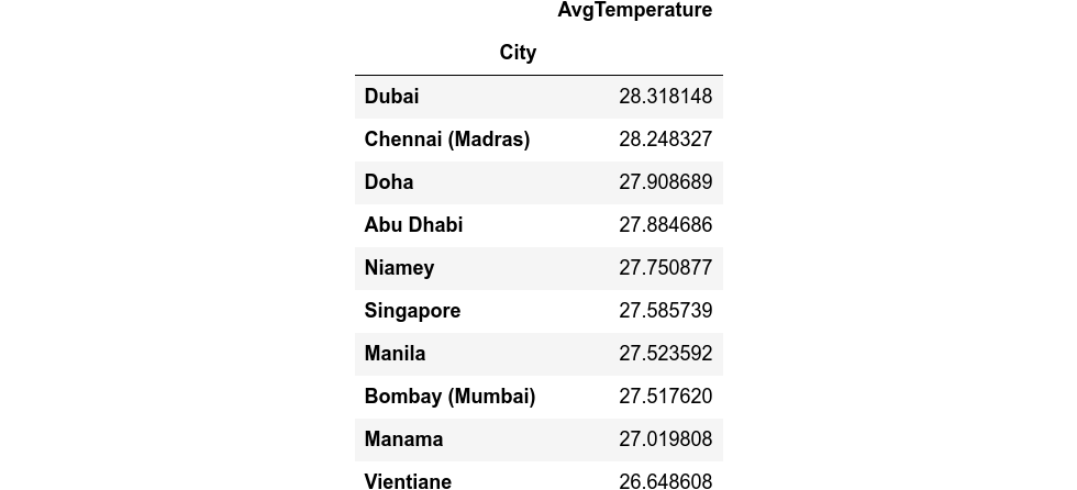

plt.figure(figsize = (12,8))
plt.barh(top_10_hotest_Cities_in_The_world.index,top_10_hotest_Cities_in_The_world.AvgTemperature)<BarContainer object of 10 artists>

4.世界上最热的城市中温度的增长 (4. The Growth of the Temperture in the hotest Cities in The world)

city_year = ['City', pd.Grouper(freq='Y')]
df_city = df.groupby(city_year).mean()
# df_city.head()plt.figure(figsize = (12,8))
for city in top_10_hotest_Cities_in_The_world.index:
    plt.plot(df_city.loc[city].index,df_city.loc[city].AvgTemperature,label = city)
plt.legend()
plt.yticks(size = 15)
plt.xticks(size = 15)
plt.ylabel("Average Temperature",size = 15)
plt.title("The Growth of the Temperture in the hotest Cities in The world",size = 20)
plt.show()

5.世界上最热的国家 (5. The hotest Countries in The world)

hotest_Countries_in_The_world = df.groupby("Country").mean().sort_values(by = "AvgTemperature")
# hotest_Countries_in_The_world.tail()plt.figure(figsize = (12,8))
plt.bar(hotest_Countries_in_The_world.index[-1:-33:-1],hotest_Countries_in_The_world.AvgTemperature[-1:-33:-1])
plt.yticks(size = 15)
plt.ylabel("Avgerage Temperature",size = 15)
plt.xticks(rotation = 90,size = 12)
plt.title("The hotest Countries in The world",size = 20)
plt.show()

7.世界平均温度¶ (7. The Average Temperature around the world¶)

when using plotly we need codes of countries Data of Codes:

当使用密谋时，我们需要国家代码代码数据：

! rm -f wikipedia-iso-country-codes.csv 
! rm -f countries-iso-codes.zip
! kaggle datasets download -d juanumusic/countries-iso-codes
! unzip countries-iso-codes.zipWarning: Your Kaggle API key is readable by other users on this system! To fix this, you can run 'chmod 600 /home/oscar/.kaggle/kaggle.json'
Downloading countries-iso-codes.zip to /home/oscar/Documentos/PYTHON/world_temperature
  0%|                                               | 0.00/4.16k [00:00<?, ?B/s]
100%|███████████████████████████████████████| 4.16k/4.16k [00:00<00:00, 879kB/s]
Archive:  countries-iso-codes.zip
  inflating: wikipedia-iso-country-codes.csvcode = pd.read_csv("wikipedia-iso-country-codes.csv") # this is for the county codes
code= code.set_index("English short name lower case")
# code.head()

I changed some countries name in the code data frame so they become the same as our main data frame index

我在代码数据框中更改了一些国家/地区名称，因此它们与我们的主要数据框索引相同

This is important when merging the two data framescode = code.rename(index={"United States Of America": "US", "Côte d'Ivoire": "Ivory Coast", 
                          "Korea, Republic of (South Korea)": "South Korea", "Netherlands": "The Netherlands", 
                          "Syrian Arab Republic": "Syria", "Myanmar": "Myanmar (Burma)",
                          "Korea, Democratic People's Republic of": "North Korea", 
                          "Macedonia, the former Yugoslav Republic of": "Macedonia", 
                          "Ecuador": "Equador", "Tanzania, United Republic of": "Tanzania", 
                          "Serbia": "Serbia-Montenegro"})
# code.head()

Now we do the merging between the code data frame and our data

现在，我们在代码数据框和我们的数据之间进行合并

hott = pd.merge(hotest_Countries_in_The_world,code,left_index = True , right_index = True , how = "left")
hott.head()

data = [dict(type="choropleth", autocolorscale=False, locations=hott["Alpha-3 code"], z=hott["AvgTemperature"],
             text=hott.index, colorscale="reds", colorbar=dict(title="Temperture"))]layout = dict(title="The Average Temperature around the world", 
              geo=dict(scope="world",
                       projection=dict(type="equirectangular"), 
                       showlakes=True, lakecolor="rgb(66,165,245)",),)fig = dict(data = data,layout=layout)
#iplot(fig,filename = "d3-choropleth-map")

8.全球12个月的平均温度变化 (8. Variation of the mean Temperature Over The 12 months around the world)

Variation_world = df.groupby(df.index.month).mean()
Variation_world = Variation_world.rename(index={1: "January", 2: "February", 3: "March", 4: "April", 5: "May",
                                                6: "June", 7: "July", 8: "August", 9: "September", 
                                                10: "October", 11: "November", 12: "December"})plt.figure(figsize=(12,8))
sns.barplot(x=Variation_world.index, y= 'AvgTemperature',data=Variation_world,palette='Set2')
plt.title('AVERAGE MEAN TEMPERATURE OF THE WORLD',size = 15)
plt.xticks(size = 10)
plt.yticks(size = 12)
plt.xlabel("Month",size = 12)
plt.ylabel("AVERAGE MEAN TEMPERATURE",size = 10)
plt.show()

9.在世界上最热的国家/地区中，过去12个月的平均温度变化：阿拉伯联合酋长国 (9. Variation of the mean Temperature Over The 12 months in the hottest country in the world: United Arab Emirates)

Variation_UAE = df.loc[df["Country"] == "United Arab Emirates"].groupby(
    df.loc[df["Country"] == "United Arab Emirates"].index.month).mean()
Variation_UAE = Variation_UAE.rename(index={1: "January", 2: "February", 3: "March", 4: "April", 5: "May",
                                            6: "June", 7: "July", 8: "August", 9: "September", 
                                            10: "October", 11: "November", 12: "December"})plt.figure(figsize=(12,8))
sns.barplot(x=Variation_UAE.index, y= 'AvgTemperature',data=Variation_UAE,palette='Set2')
plt.title('Variation of the mean Temperature Over The 12 months in the United Arab Emirates',size = 20)
plt.xticks(size = 10)
plt.yticks(size = 12)
plt.xlabel("Month",size = 12)
plt.ylabel("AVERAGE MEAN TEMPERATURE",size = 12)
plt.show()

10.每个区域几个月内的平均温度变化 (10. Variation of mean Temperature over the months for each region)

plt.figure(figsize=(12, 18))
i = 1  # this is for the subplot
for region in df.Region.unique():  # this for loop make it easy to visualize every region with less code
    region_data = df[df['Region'] == region]
    final_data = region_data.groupby(region_data.index.month).mean()[
        'AvgTemperature'].sort_values(ascending=False)
    final_data = pd.DataFrame(final_data)
    final_data = final_data.sort_index()
    final_data = final_data.rename(index={1: "January", 2: "February", 3: "March", 4: "April", 5: "May",
                                          6: "June", 7: "July", 8: "August", 9: "September",
                                          10: "October", 11: "November", 12: "December"})
    plt.subplot(4, 2, i)
    sns.barplot(x=final_data.index, y='AvgTemperature',
                data=final_data, palette='Paired')
    plt.title(region, size=10)
    plt.xlabel(None)
    plt.xticks(rotation=90, size=9)
    plt.ylabel("Mean Temperature", size=11)
    i += 1

1. The Average Temperature in Spain
   西班牙的平均温度

Average_Temperature_Spain = df.loc[df["Country"] == "Spain"].groupby("City").mean()
Average_Temperature_Spain.head()

Average_Temperature_USA = df.loc[df["Country"] == "US"].groupby("State").mean().drop(["Additional Territories"],
                                                                                     axis = 0)
# Average_Temperature_USA.head()

we need to add the code to this data for visualization

我们需要向该数据添加代码以进行可视化

! rm -f state-areas.csv
! rm -f state-population.csv
! rm -f state-abbrevs.csv
! rm -f usstates-dataset.zip
! kaggle datasets download -d giodev11/usstates-dataset
! unzip usstates-dataset.zipWarning: Your Kaggle API key is readable by other users on this system! To fix this, you can run 'chmod 600 /home/oscar/.kaggle/kaggle.json'
Downloading usstates-dataset.zip to /home/oscar/Documentos/PYTHON/world_temperature
  0%|                                               | 0.00/18.4k [00:00<?, ?B/s]
100%|██████████████████████████████████████| 18.4k/18.4k [00:00<00:00, 2.38MB/s]
Archive:  usstates-dataset.zip
  inflating: state-abbrevs.csv       
  inflating: state-areas.csv         
  inflating: state-population.csvusa_codes = pd.read_csv('state-abbrevs.csv')
# Duplicate columns
usa_codes['State'] = usa_codes['state']
# Set new index
usa_codes =usa_codes.set_index("State")
# Rename columns
usa_codes.rename(columns={'abbreviation': 'Code', 'state': 'State'}, inplace=True)Average_Temperature_USA = pd.merge(Average_Temperature_USA,
                                   usa_codes,how = "left",right_index = True,left_index = True)
Average_Temperature_USA.head()

data_usa = [dict(type="choropleth", autocolorscale=False, locations=Average_Temperature_USA["Code"],
                 z=Average_Temperature_USA["AvgTemperature"],
                 locationmode="USA-states",
                 text=Average_Temperature_USA.index, colorscale="reds", colorbar=dict(title="Temperture"))]
layout_usa = dict(title="The Average Temperature in the USA states", 
                  geo=dict(scope="usa", projection=dict(type="albers usa"), 
                           showlakes=True, lakecolor="rgb(66,165,245)",),)fig_usa = dict(data = data_usa,layout=layout_usa)
#iplot(fig_usa,filename = "d3-choropleth-map")

12，1995年至2020年美国平均气温 (12.Average Temperature in USA from 1995 to 2020)

Temperature_USA_year = df.loc[df["Country"] == "US"].groupby(pd.Grouper(freq = "Y")).mean()
#Temperature_USA_year.head()plt.figure(figsize = (12,8))
sns.barplot(x = Temperature_USA_year.index.year,y = "AvgTemperature",data = Temperature_USA_year)
plt.yticks(size = 12)
plt.xticks(size = 12,rotation = 90)
plt.xlabel(None)
plt.ylabel("Avgerage Temperature",size = 12)
plt.title("Average Temperature in USA from 1995 to 2020",size = 15)
plt.show()

结论 (Conclusion)

Displaying the data via plots can be an effective way to quickly present the data.

通过绘图显示数据是快速显示数据的有效方法。

I hope it will help you to develop your training.

我希望它能帮助您发展培训。

No matter what books or blogs or courses or videos one learns from, when it comes to implementation everything might look like “Out of Syllabus”

无论从中学到什么书，博客，课程或视频，到实施时，一切都可能看起来像“课程提纲”

Best way to learn is by doing!

最好的学习方法就是干！

Best way to learn is by teaching what you have learned!

最好的学习方法是教您所学的知识！

永不放弃！ (Never give up!)

See you in Linkedin!

在Linkedin上见！

翻译自: https://medium.com/swlh/working-with-temperatures-6133baa35a7c

绝缘子工作温度