介绍 (Introduction)
It's pretty rare to apply machine learning to a real-world problem and you have something as straightforward as you might find in tutorials or in data science courses. A lot of the time you come across classification problems where you are trying to predict something that does not occur very often. This is common when trying to predict things like conversion, churn, fraud. In this post, I am going to talk about class imbalances in machine learning. In particular, I want to go over some of the implications of having imbalanced data as well as highlight and explain some ways to address it. My hope is that by the end of this post you will have the tools you need to handle this issue in any prediction problems you may come across.
很难将机器学习应用于现实世界中的问题,并且您会像在教程或数据科学课程中发现的那样简单明了。 很多时候,您会遇到分类问题,在这些问题中您试图预测很少发生的事情。 在尝试预测转化,流失,欺诈等情况时,这很常见。 在这篇文章中,我将讨论机器学习中的课堂失衡。 特别是,我想讲解数据不平衡的一些含义,并强调并解释一些解决方法。 我希望到本文结束时,您将拥有处理可能遇到的任何预测问题所需的工具。
什么是不平衡数据,为什么会出现问题? (What is imbalanced data and why is it a problem?)
Like I said above, imbalanced data comes about when we have significant differences in the proportion of the class we are trying to predict. For example, in a lot of industries, customer churn over a certain period of time would be relatively rare (hopefully). If we try and formulate a machine learning model to predict whether a customer will churn or not we might only have 5 per cent of customers churning and 95 per cent not churning. For something like conversion or fraud, this is probably going to be even lower.
就像我在上面说过的那样,当我们试图预测的班级比例有显着差异时,就会出现数据不平衡的情况。 例如,在许多行业中,在一定时期内客户流失是相对罕见的(希望如此)。 如果我们尝试建立一个机器学习模型来预测客户是否会流失,那么我们可能只有5%的客户流失,而95%的客户流失。 对于诸如转换或欺诈之类的事情,这可能会更低。
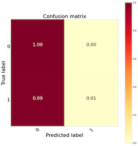
Ok so the problem is hopefully a little bit clearer, but why do we care? Let's just train the model and make some predictions. Let's take the churn example in the above paragraph and estimate a logistic regression. After estimating the model we get 95 per cent of the predictions correct. That was easy. If we dig a bit deeper into the results, however, and look at the confusion matrix, we might find something like Figure 1 below. Our model predicted that basically nobody churned. That isn't very helpful, we could have made that prediction ourselves and saved ourselves the trouble of writing any code. Obviously, this model is pretty useless and not really adding any value. What's going on here? Why is our model so bad? The training set is so unbalanced that the model has a hard time finding useful patterns in the minority class. This is more pronounced with some algorithms such as logistic regression as it assumes the class distributions are equal. Lucky for us, there are several ways to deal with this and this is what I will be going through in this post.
好的,希望这个问题可以解决一些,但是为什么我们要关心呢? 让我们只训练模型并做出一些预测。 让我们以上段中的流失示例为例,并估计逻辑回归。 估计模型后,我们得到了95%的正确预测。 那很简单。 但是,如果我们对结果进行更深入的研究,然后查看混淆矩阵,则可能会发现下面的图1所示的内容。 我们的模型预测基本上没有人搅动。 那不是很有帮助,我们可以自己进行预测并节省编写任何代码的麻烦。 显然,该模型是没有用的,并没有真正增加任何价值。 这里发生了什么? 为什么我们的模型这么差? 训练集非常不平衡,以至于该模型很难在少数群体中找到有用的模式。 这在某些算法(例如逻辑回归)中更为明显,因为它假设类分布相等。 对我们来说幸运的是,有几种方法可以解决这个问题,这就是我将在本文中介绍的内容。
采样技术 (Sampling Techniques)
The first potential solution we could try is to resample our data to balance the classes. There are a few different sampling methods we could try all of which can be easily implemented in the imblearn python library.
我们可以尝试的第一个潜在解决方案是对数据重新采样以平衡类。 我们可以尝试几种不同的采样方法,所有这些方法都可以在imblearn python库中轻松实现。
One key point to mention is that these re-sampling techniques should only be performed on the training data. The test set should remain unbalanced.
要提到的一个关键点是,这些重采样技术应仅在训练数据上执行。 测试仪应保持不平衡。
To start off our analysis lets first use a handy function from sklearn to create a dataset. The make_classification function is really useful and allows us to create a dataset to demonstrate these techniques and algorithms. Notice, we have added weights=[0.99,0.01] to the arguments to generate an unbalanced dataset. This level of unbalance is very similar to a machine learning project I worked on recently and is not that uncommon to see datasets like these in practice.
首先,我们首先使用sklearn中的便捷功能来创建数据集。 make_classification函数非常有用,它允许我们创建一个数据集来演示这些技术和算法。 注意,我们在参数中增加了weight = [0.99,0.01]以生成不平衡数据集。 这种不平衡程度与我最近从事的机器学习项目非常相似,并且在实践中看到这样的数据集并不少见。
from sklearn.datasets import make_classification
X,y = make_classification(n_samples=10000, n_features=2, n_informative=2,
                          n_redundant=0, n_repeated=0, n_classes=2,
                          n_clusters_per_class=1,class_sep=1,
                          flip_y=0, weights=[0.99,0.01], random_state=17)
随机欠采样 (Random Undersampling)
First off, let's take a look at undersampling. This technique is pretty simple and involves randomly selecting samples from the majority class and using these along with our minority class for training data. The result is we end up with an equal number of positive and negative examples which can avoid the problems outlined above. The advantage of this technique is that is pretty easy to implement and it can be quite effective. The downside is that you are essentially throwing away data. I would probably not favour this approach unless my training data was quite large and I could afford to throw away data. In Figure 2 below we can see the code to implement this as well as our training set after undersampling. Notice how much data we have removed.
首先,让我们看一下欠采样。 该技术非常简单,涉及从多数类中随机选择样本,并将其与我们的少数类一起用于训练数据。 结果是我们得到了相等数量的正面和负面例子,可以避免上面概述的问题。 该技术的优点是非常容易实现并且非常有效。 缺点是您实际上是在丢弃数据。 除非我的训练数据很大并且我有能力丢弃数据,否则我可能不会赞成这种方法。 在下面的图2中,我们可以看到实现此功能的代码以及欠采样后的训练集。 注意我们删除了多少数据。
from imblearn.under_sampling import RandomUnderSampler
undersamp = RandomUnderSampler(random_state=1)
X_over, y_over = undersamp.fit_resample(X, y)
f, axes = plt.subplots(1, 2, figsize=(12,10))
sns.scatterplot(X[:,0],X[:,1],hue=y, ax=axes[0]);
sns.scatterplot(X_over[:,0],X_over[:,1],hue=y_over, ax=axes[1]);
随机过采样 (Random Oversampling)
Oversampling is the opposite of undersampling. With this approach, we randomly sample data from the minority class and duplicate it to create more samples. We do this until the class distribution is equal. Although this can be useful for addressing imbalances, it has some disadvantages as well. The major one being that we are duplicating already existing data. This means we are not really adding any additional information to the classification problem and it can potentially lead to overfitting which is definitely something we want to avoid.
过采样与欠采样相反。 使用这种方法,我们可以对少数群体的数据进行随机抽样,然后将其复制以创建更多样本。 我们这样做直到类分布相等为止。 尽管这对于解决不平衡很有用,但也有一些缺点。 主要的是我们正在复制已经存在的数据。 这意味着我们没有真正在分类问题上添加任何其他信息,并且有可能导致过度拟合,这绝对是我们要避免的事情。
from imblearn.over_sampling import RandomOverSampler
oversamp = RandomOverSampler(random_state=1)
X_over, y_over = oversamp.fit_resample(X, y)


f, axes = plt.subplots(1, 2, figsize=(12,10))
sns.scatterplot(X[:,0],X[:,1],hue=y, ax=axes[0]);
sns.scatterplot(X_over[:,0],X_over[:,1],hue=y_over, ax=axes[1]);
SMOTE(合成少数族裔过采样技术) (SMOTE (Synthetic Minority Over-sampling TEchnique))
As the name implies, SMOTE is an oversampling method used to generate additional data from the data we already have. It is similar to random oversampling but rather than duplicate existing data we are generating new synthetic data. The original paper describes the technique as follows:
顾名思义,SMOTE是一种过采样方法,用于从我们已有的数据中生成其他数据。 它类似于随机过采样,但不是复制现有数据,而是生成新的合成数据。 原始论文对此技术进行了如下描述:
“The minority class is over-sampled by taking each minority class sample and introducing synthetic examples along the line segments joining any/all of the k minority class nearest neighbours”.
“通过获取每个少数族裔样本并沿连接任何/全部k个少数族裔最近邻的线段引入综合示例,对少数族裔进行了过度采样”。
So what does this mean? well, the algorithm first uses k-nearest neighbours to decide which data points we are going to use to produce new data. For simplicity, let's say we choose k = 1. The algorithm will create a line segment between our data point at its nearest neighbour and produce a new data point somewhere along this line. Let's say the feature we are generating data for is the number of days since a user last visited our website. To generate new synthetic data, the algorithm computes two new variables. The gap which is a random number between 0 and 1 let's say we get 0.8, and the diff, which is the difference between the number of days since a user last visited for our first data point (20) and its nearest neighbour (15). The value of our synthetic data for this feature is then: 24= 20+ (20–15)*.8.
那么这是什么意思? 很好,该算法首先使用k最近邻来决定我们将使用哪些数据点来生成新数据。 为简单起见,假设我们选择k =1。该算法将在我们数据点的最近邻居处创建一条线段,并沿着该线在某处生成一个新数据点。 假设我们生成数据的功能是自用户上次访问我们网站以来的天数。 为了生成新的合成数据,该算法计算了两个新变量。 差距是0到1之间的一个随机数,假设我们得到0.8,而diff是用户自上次访问我们的第一个数据点(20)到其最近邻居(15)以来的天数之差。 。 那么我们为此功能合成的数据值为:24 = 20+(20–15)*。8。
Ok, let's see how we can implement this in python and also visualise what the algorithm produces. You might think the graph looks a bit strange and I would probably agree but this is just an artefact of the algorithm and reinforces that the data is ‘synthetic’ rather than completely new as it directly depends on the other data points (or at least its nearest data points).
好的,让我们看看如何在python中实现它,并可视化算法产生的结果。 您可能会认为该图看起来有些奇怪,我可能会同意,但这只是算法的一种伪像,它强调了数据是“合成的”而不是全新的,因为它直接依赖于其他数据点(或至少依赖于其他数据点)。最近的数据点)。
from imblearn.over_sampling import SMOTE
ax = plt.figure(figsize=(10,8))
sns.scatterplot(X[:,0],X[:,1],hue=y);
oversample = SMOTE()
X, y = oversample.fit_resample(X, y)
ax = plt.figure(figsize=(10,8))
sns.scatterplot(X[:,0],X[:,1],hue=y);
There are pros and cons to each of these techniques but in practice, I would recommend trying all of them to see which works best and let your model metrics guide you.
这两种技术各有优缺点,但在实践中,我建议尝试所有这些技术,看看哪种方法最有效,并让您的模型指标为您提供指导。
Here is a link to the full paper for those of you more interested in the details: https://arxiv.org/pdf/1106.1813.pdf
对于那些对细节感兴趣的人,这里是全文的链接: https : //arxiv.org/pdf/1106.1813.pdf
类权重 (Class Weighting)
As I mentioned above, many machine learning algorithms assume that the class distribution is equal so they may not work very well out of the box. This is the case for something like logistic regression. To get around that there is a nice argument called class_weights in sklearn which lets us tell the model what the class distribution is. It is a simple and effective solution and I have found good success with it in the past. To be more specific, it will penalise the model more for making mistakes on the minority class. These mistakes will make it harder to minimise the cost function so the model learns to put more emphasis on getting the minority class correct.
如前所述,许多机器学习算法都假设类分布相等,因此开箱即用时效果可能不佳。 逻辑回归之类的情况就是这种情况。 为了解决这个问题,在sklearn中有一个很好的参数class_weights ,它可以让我们告诉模型类的分布是什么。 这是一个简单有效的解决方案,过去我已经获得了很好的成功。 更具体地说,由于在少数群体上犯错误,它将对模型造成更多的惩罚。 这些错误将使将成本函数最小化变得更加困难,因此该模型将学习更多地强调正确设置少数群体。
The code below shows how we can implement this in python. We can either choose class_weight = ‘balanced’ or pass a dictionary with specific class weights, e.g. weights = {0:0.01, 1:1.0}
下面的代码显示了我们如何在python中实现这一点。 我们可以选择class_weight ='balanced'或通过具有特定类别权重的字典,例如weights = {0:0.01,1:1.0}
from sklearn.linear_model import LogisticRegression
from sklearn.model_selection import train_test_split
x_train, x_test, y_train, y_test = train_test_split(X, y, random_state=1, test_size=0.3)
lr = LogisticRegression(class_weight='balanced')
lr.fit(x_train, y_train)
With a variety of techniques presented and explained to you, I thought I would also share an interesting conversation I had with a colleague when discussing imbalanced data. He made the point that:
通过向您介绍和向您介绍各种技术,我想我也将在讨论不平衡数据时与同事分享一个有趣的对话。 他指出:
Imbalanced data does not really matter when using a model such as logistic regression in so far as it does not affect the coefficient estimates (only the intercept).
当使用逻辑回归等模型时,不平衡数据并不重要,只要它不影响系数估计(仅截距)即可。
The intercept will adjust to the imbalance and the coefficients will remain the same. After thinking about it, I realised that he was right. There is one problem with this, however. If you plot the distribution of the prediction probabilities you will likely see a very skewed distribution. For example, when I did this my distribution ranged from 0 to ~0.2. This for me is a problem particularly when the outputs of the model need to be interpreted and explained to the business teams in your company. For this reason alone I think it is much better to re-balance the data even though in principle a logistic regression can handle imbalances.
截距将调整为不平衡,系数将保持不变。 考虑了一下,我意识到他是对的。 但是,这有一个问题。 如果绘制预测概率的分布图,则可能会看到非常偏斜的分布。 例如,当我这样做时,我的分布范围从0到〜0.2。 对于我来说,这尤其是一个问题,当需要向公司中的业务团队解释和解释模型的输出时。 仅出于这个原因,我认为重新平衡数据要好得多,即使原则上逻辑回归可以处理不平衡问题。
算法和指标 (Algorithms and Metrics)
As I alluded to earlier, the choice of algorithm can also greatly impact your results when dealing with imbalanced data. It is also very important to choose appropriate metrics to assess the performance of your model. Again, accuracy would not be a particularly useful metric to consider in this case. Using metrics such as ROC AUC, Precision and Recall and the confusion matrix will give us a much better idea of how the model is performing.
正如我之前提到的,在处理不平衡数据时,算法的选择也会极大地影响您的结果。 选择适当的指标来评估模型的性能也很重要。 同样,在这种情况下,精度不是要考虑的特别有用的指标。 使用ROC AUC,Precision和Recall等指标以及混淆矩阵将使我们对模型的性能有更好的了解。
I won't dive too deep into how these metrics work here but here are some resources which go into detail for each of these metrics.
我不会在这里深入探讨这些指标的工作原理,但是这里有一些资源针对这些指标进行了详细介绍。
测试不同的方法 (Testing the different methods)
Alright, that is enough of the background stuff, let’s get to the interesting part and look at an example of this with some code. I recently had to apply these techniques in a project and they worked reasonably well for me. Unfortunately, as the data is sensitive I can’t show it but we can re-create a similar scenario by generating some data. In any case, the techniques and the code I show here should be readily transferable to other classification problem. Below we will estimate a few different models and see how they perform on the unbalanced dataset. We will then try out the techniques above and see how they improve our results using some key classification performance metrics.
好了,这已经足够了背景知识,让我们进入有趣的部分,并使用一些代码查看其中的一个示例。 我最近不得不在项目中应用这些技术,并且它们对我来说相当不错。 不幸的是,由于数据很敏感,我无法显示它,但是我们可以通过生成一些数据来重新创建类似的场景。 无论如何,我在这里显示的技术和代码应该可以容易地转移到其他分类问题。 下面我们将估计一些不同的模型,并查看它们在不平衡数据集上的表现。 然后,我们将尝试上述技术,并使用一些关键的分类性能指标来查看它们如何改善我们的结果。
生成数据进行建模 (Generating Data For Modelling)
Again we can use the make_classification function in sklearn to create our imbalanced dataset. For this example, we will have 1 per cent positive examples and 99 per cent negative examples.
同样,我们可以在sklearn中使用make_classification函数来创建不平衡数据集。 对于此示例,我们将有1%的正面示例和99%的负面示例。
from sklearn import datasets
from collections import Counter


X, y = datasets.make_classification(
            n_samples     = 100000,  # number of data points
            n_classes     = 2,      # number of classes
            n_clusters_per_class=2, # The number of clusters per class
            weights       = [0.99,0.01], # The proportions assigned to each class
            n_features    = 12,     # number of total features
            n_informative = 5,      # number of informative features
            n_redundant   = 7,      # number of redundant features
            class_sep=0.9,
            random_state  = 0                       )
print('Original dataset shape {}'.format(Counter(y)))
Imblearn管道 (Imblearn Pipelines)
To estimate these models using different sampling techniques we will make use of imblearn pipelines. I'm sure some of you have heard of sklearn pipelines, and these are essentially the same but designed to specifically work with sampling techniques. As far as I know, it is not possible to use these sampling techniques with sklearn pipelines currently. This is my first time using pipelines and I have to say they make your code much cleaner and easier to read. They are pretty handy so I will definitely incorporate these into my workflow going forward.
为了使用不同的采样技术估算这些模型,我们将使用imblearn管道。 我敢肯定,有些人听说过sklearn管道,这些管道基本相同,但专门用于采样技术。 据我所知,目前无法将这些采样技术与sklearn管道一起使用。 这是我第一次使用管道,我不得不说它们使您的代码更加简洁和易于阅读。 它们非常方便,因此我一定会在以后的工作流程中将它们合并。
To use these pipelines, all we need to do is create an instance of our sampling class and our algorithm and then pass these as tuples into the pipeline class. I originally tried to see if I could pass multiple algorithms into the pipeline, i.e. logistic regression and random forest but this did not work. However, if you pass algorithms with a fit a transform method such as PCA it should work fine. From the imblearn docs:
要使用这些管道,我们所需要做的就是创建采样类和算法的实例,然后将它们作为元组传递到管道类中。 我最初试图查看是否可以将多种算法传递到管道中,即逻辑回归和随机森林,但这是行不通的。 但是,如果通过适合的转换方法(例如PCA)传递算法,则应该可以正常工作。 从imblearn文档中:
Intermediate steps of the pipeline must be transformers or resamplers, that is, they must implement fit, transform and sample methods.
管道的中间步骤必须是转换器或重采样器,也就是说,它们必须实现拟合,变换和采样方法。
Logistic回归管道代码 (Code for logistic Regression Pipeline)
from imblearn.pipeline import make_pipeline, Pipeline
from imblearn.under_sampling import RandomUnderSampler
from imblearn.over_sampling import RandomOverSampler
from imblearn.over_sampling import SMOTE


undersamp = RandomUnderSampler(random_state=1)
oversamp = RandomOverSampler(random_state=1)
smote = SMOTE()


lr = LogisticRegression()


# pipeline for each type of sampler
pipeline_0 = Pipeline([('lr', lr)])
pipeline_1 = Pipeline([('undersamp', undersamp), ('lr', lr)])
pipeline_2 = Pipeline([('oversamp', oversamp), ('lr', lr)])
pipeline_3 = Pipeline([('smote', smote), ('lr', lr)])


## Split train and test
x_train, x_test, y_train, y_test = train_test_split(X, y, random_state=1, test_size=0.25,
                                                    stratify=y)


# loop to run all pipelines
pipeline_list = [pipeline_0, pipeline_1, pipeline_2, pipeline_3]
for num, pipeline in enumerate(pipeline_list):
    print("Estimating Pipeline {}".format(num))
    pipeline.fit(x_train, y_train)
    y_pred = pipeline.predict(x_test)
    probs = pipeline.predict_proba(x_test)[:,1]
    print("Confusion Matrix for pipeline {}:".format(num))
    print(confusion_matrix(y_test, y_pred))


    cm = confusion_matrix(y_test, y_pred)
    plot_confusion_matrix(cm, classes = [0, 1])
    plot_confusion_matrix(cm, classes = [0, 1], normalize=True)


    plot_roc_curve(y_test, probs)
    plot_precision_recall(y_test, probs)
随机森林管道规范 (Code for Random Forest Pipeline)
from imblearn.pipeline import Pipeline
from imblearn.under_sampling import RandomUnderSampler
from imblearn.over_sampling import RandomOverSampler
from imblearn.over_sampling import SMOTE
from sklearn.ensemble import RandomForestClassifier


undersamp = RandomUnderSampler(random_state=1)
oversamp = RandomOverSampler(random_state=1)
smote = SMOTE()


rf = RandomForestClassifier(random_state=88, n_estimators=500,
                            criterion='entropy', max_depth=8,
                            max_features='auto')


# pipeline for each type of sampler
pipeline_0 = Pipeline([('rf', rf)])
pipeline_1 = Pipeline([('undersamp', undersamp), ('rf', rf)])
pipeline_2 = Pipeline([('oversamp', oversamp), ('rf', rf)])
pipeline_3 = Pipeline([('smote', smote), ('rf', rf)])


# loop to run all pipelines
pipeline_list = [pipeline_0, pipeline_1, pipeline_2, pipeline_3]
for num, pipeline in enumerate(pipeline_list):
    print("Estimating Pipeline {}".format(num))
    pipeline.fit(x_train, y_train)
    y_pred = pipeline.predict(x_test)
    probs = pipeline.predict_proba(x_test)[:,1]
    print("Confusion Matrix for {} Model:".format(num))
    print(confusion_matrix(y_test, y_pred))


    cm = confusion_matrix(y_test, y_pred)
    plot_confusion_matrix(cm, classes = [0, 1])
    plot_confusion_matrix(cm, classes = [0, 1], normalize=True)


    plot_roc_curve(y_test, probs)
    plot_precision_recall(y_test, probs)
结果 (Results)
逻辑回归 (Logistic Regression)
数据不平衡 (Unbalanced Data)

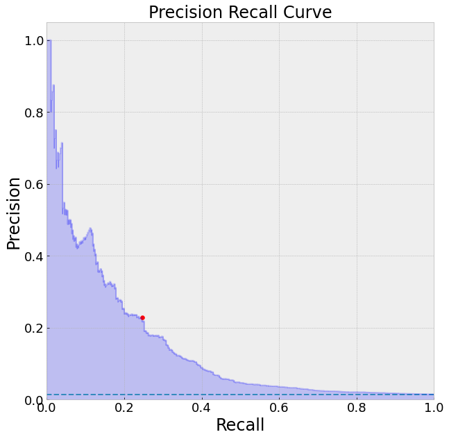

We can see that the results from our unbalance dataset are not that great. The model with a threshold of 0.5 performs very badly identifying nearly none of our positive examples. We could try and alter the threshold appropriately but again this will give us very skewed probabilities as outputs. We can also see from our PR-curve that the model has a hard time identifying the positive labels without making a lot of mistakes. Interestingly, the ROC actually seems to look fine. This highlights that ROC can be a misleading metric when dealing with unbalanced data. To see what's happening here, think about what the ROC is plotting, the true positive rate (TPR) vs the false positive rate (FPR). Below are the definitions of TPR and FPR.
我们可以看到不平衡数据集的结果不是很好。 阈值为0.5的模型很难很好地识别我们的正例。 我们可以尝试适当地更改阈值,但是这又会给我们带来非常偏差的概率作为输出。 我们还可以从PR曲线中看到,该模型很难确定正标签,而不会犯很多错误。 有趣的是,中华民国实际上看起来还不错。 这突出表明,在处理不平衡数据时,ROC可能是误导性指标。 要查看此处发生的情况,请考虑一下ROC所绘制的内容,即真实阳性率(TPR)对假阳性率(FPR)。 以下是TPR和FPR的定义。
Recall/TPR = TP / (TP+FN)
召回/ TPR = TP /(TP + FN)
FPR = FP / (FP + TN)
FPR = FP /(FP + TN)
Because our classes are imbalanced we have far more negative examples. In essence, our model is biased towards predicting negative examples so we have a lot of True negatives (TN). This keeps our false positive rate (FPR) from increasing too much since our TN will be increasing in the denominator. This is why we can get a high AUC even if we are doing a bad job at classifying the positive examples (the ones we care about most). If we use precision and recall, however, this problem is avoided since we are not using the True negatives (TN) at all.
由于班级不平衡,我们有更多负面的例子。 从本质上讲,我们的模型偏向于预测否定实例,因此我们有很多真实否定(TN)。 这可以防止我们的误报率(FPR)增加过多,因为我们的TN分母将增加。 这就是为什么即使在分类正面示例(我们最关心的示例)方面做得很差的情况下,我们也可以获得较高的AUC的原因。 但是,如果我们使用精度和查全率,则可以避免此问题,因为我们根本没有使用真负片(TN)。
Precision = TP/(TP+FP)
精度= TP /(TP + FP)
Recall/TPR = TP/(TP+FN)
召回/ TPR = TP /(TP + FN)
In this case, my preference is to use the confusion matrix and to a lesser extent the PR-curve to gauge the performance of the model. Note I make use of a few helper functions that I created to plot these metrics. The code is located at the bottom of this post. All of the figures presented use the default thresholds of 0.5. This can easily be altered to adjust the predictions as required, depending on your use case.
在这种情况下,我更喜欢使用混淆矩阵,并在较小程度上使用PR曲线来评估模型的性能。 注意我使用了一些创建的辅助功能来绘制这些度量。 该代码位于此帖子的底部。 呈现的所有图均使用默认阈值0.5。 根据您的用例,可以轻松更改此值以根据需要调整预测。
What about our sampling methods?
那我们的采样方法呢?
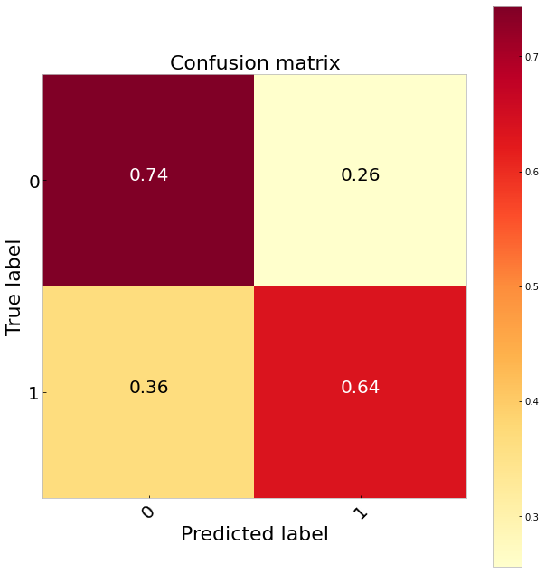
Overall, the results are pretty much the exact same across different sampling methods. So what should we do in this case? In general these results arent great so at this point, I would suggest experimenting with other models. But if we were determined to estimate a logistic regression and we had a large data set we could favour undersampling since it is the least complex of the three options and try and optimise our decision threshold to improve our TP rate.
总体而言,不同采样方法的结果几乎完全相同。 那么在这种情况下我们该怎么办? 总的来说,这些结果都很好,所以在这一点上,我建议尝试使用其他模型。 但是,如果我们决心估计逻辑回归,并且拥有大量数据集,那么我们可能会偏低采样率,因为这是三种选择中最复杂的一种,并尝试优化决策阈值以提高目标利率。
欠采样 (Undersampling)


过采样 (Oversampling)


冒烟 (SMOTE)


随机森林 (Random Forest)
So logistic regression didn't perform too well at this problem, how about we try a random forest. These models tend to perform well in practice and they are usually my go-to model for classification problems. As for the results, this model performs slightly better than the logistic regression on the unbalanced data at the default threshold identifying 9 per cent of the TP’s. Obviously we want something a bit better than this so let's try our sampling techniques again.
因此,逻辑回归在此问题上的表现不是很好,我们如何尝试随机森林。 这些模型在实践中往往表现良好,它们通常是分类问题的首选模型。 至于结果,该模型在默认阈值(标识了TP的9%)下对不平衡数据的逻辑回归性能略好于Logistic回归。 显然,我们希望有比这更好的东西,所以让我们再次尝试采样技术。
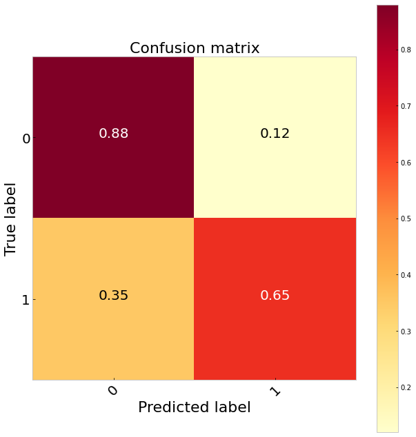
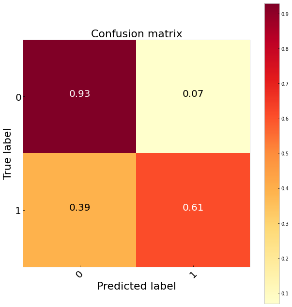
Comparing the three sampling methods suggests undersampling performs the best classifying 65 per cent of the true positives. It also does a much better job identifying the true negatives than the logistic regression. Our best results, however, come from balancing the class weights. Since this is very simple to do in sklearn (class_weights = ‘balanced’) and we do not have to throw any data away this would be my preference. Doing this gives us a 70 per cent TP rate.
比较这三种采样方法表明,欠采样对65%的真实阳性的分类效果最好。 与逻辑回归相比,它在识别真正的负面因素方面做得更好。 但是,我们最好的结果来自平衡班级权重。 因为这在sklearn中非常简单(class_weights ='balanced'),并且我们不必丢弃任何数据,所以这是我的偏爱。 这样做使我们的目标价率为70%。
What else could we do to improve the model score?
我们还能做些什么来提高模型分数?
There are a few other things we could try here to improve our model performance as well as make sure our predictions are robust.
我们还可以尝试其他一些方法来改善我们的模型性能,并确保我们的预测是可靠的。
KFold Cross-validation: I did not perform cross-validation here but I would recommend it. It is really simple using sklearn using cross_val_score.
KFold交叉验证:我在这里没有执行交叉验证,但我建议这样做。 使用sklearn和 cross_val_score 真的很简单 。
Other models: SVM, lightGBM, XGBoost to name a few.
其他型号:SVM,lightGBM,XGBoost等。
Hyperparameter Optimisation: this can be particularly useful for models with many hyperparameters.
超参数优化 :这对于具有许多超参数的模型特别有用。
欠采样 (Undersampling)


过采样 (Oversampling)


冒烟 (SMOTE)


类权重 (Class Weights)


主要要点 (Main Takeaways)
So what can we take away from these examples?
那么我们可以从这些例子中拿走什么呢?
There are many ways to address the problem of imbalanced data and the effectiveness of each will likely depend on your problem and data.
解决数据不平衡问题的方法很多,每种方法的有效性可能取决于您的问题和数据。
Choosing appropriate metrics for the specific problem is important: I would recommend looking at more than one. No one metric is perfect.
为特定问题选择适当的指标很重要:我建议您考虑多个指标。 没有一个指标是完美的。
Trying multiple algorithms can give much better results: each has its own advantages and disadvantages: e.g. random forest often perform better but can be harder to interpret than logistic regression, they are also more computationally complex.
尝试多种算法会产生更好的结果:每种算法都有其自身的优缺点:例如,随机森林通常表现更好,但比逻辑回归更难解释,它们的计算复杂度也更高。
Not re-balancing data can give very skewed output probabilities which can be difficult to interpret and explain.
不重新平衡数据可能会产生非常不正确的输出概率,这可能很难解释和解释。
Altering thresholds can also be effective: how much you alter them will depend on the relative costs of your model making mistakes.
更改阈值也可能有效:更改阈值的多少取决于模型出错的相对成本。
Ok, guys that is it for this post, as always thanks for reading and I hope you found this useful.
好的,伙计们,就是这篇文章,一如既往地感谢您的阅读,我希望您觉得这篇文章有用。
辅助函数的Python代码 (Python Code for Helper Functions)
Below are some useful functions to help us assess our model performance.
以下是一些有用的功能,可帮助我们评估模型的性能。
def plot_precision_recall(test_y, probs, title='Precision Recall Curve', threshold_selected=None):
    """Plots precision recall curve

    """
    precision, recall, threshold = precision_recall_curve(test_y, probs)
    plt.figure(figsize=(10, 10))
    no_skill = len(test_y[test_y==1]) / len(test_y)
    plt.plot([0,1], [no_skill,no_skill], linestyle='--', label='Random')


    step_kwargs = ({'step': 'post'})
    plt.step(recall, precision, color='b', alpha=0.2,
             where='post')
    plt.fill_between(recall, precision, alpha=0.2, color='b', **step_kwargs)


    fscore = (2 * precision * recall) / (precision + recall)


    ix = np.argmax(fscore)
    print('Best Threshold=%f, F-Score=%.3f' % (threshold[ix], fscore[ix]))
    plt.scatter(recall[ix], precision[ix], marker='o', color='red', label='Best')


    plt.xlabel('Recall', size=24)
    plt.ylabel('Precision', size=24)
    plt.ylim([0.0, 1.05])
    plt.xlim([0.0, 1.0])
    plt.title(title, size=24)
    plt.xticks(size=18)
    plt.yticks(size=18)


    if threshold_selected:
        p = precision[np.where(threshold == threshold_selected)[0]]
        r = recall[np.where(threshold == threshold_selected)[0]]
        plt.scatter(r, p, marker='*', s=600, c='r')
        plt.vlines(r, ymin=0, ymax=p, linestyles='--')
        plt.hlines(p, xmin=0, xmax=r, linestyles='--')
        plt.text(r - 0.1, p + 0.15,
                 s='Threshold: '+round(threshold_selected, 2), size=20, fontdict={'weight': 1000})
        plt.text(r - 0.2, p + 0.075,
                 s='Precision: ' + round(100 * p[0], 2)+'Recall: ' + round(100 * r[0], 2), size=20,
                 fontdict={'weight': 1000})


    pr = pd.DataFrame({'precision': precision[:-1], 'recall': recall[:-1],
                       'threshold': threshold})
    return pr


def plot_confusion_matrix(cm, classes,
                          normalize=False,
                          title='Confusion matrix',
                          cmap=plt.cm.YlOrRd):
    """
        Plots the confusion matrix either numbers or proportions
    """
    if normalize:
        cm = cm.astype('float') / cm.sum(axis=1)[:, np.newaxis]
        print("Normalized confusion matrix")
    else:
        print('Confusion matrix, without normalization')


    print(cm)
    plt.style.use('bmh')
    plt.figure(figsize=(9, 9))
    plt.imshow(cm, interpolation='nearest', cmap=cmap)
    plt.title(title, size=22)
    plt.colorbar()
    tick_marks = np.arange(len(classes))
    plt.xticks(tick_marks, classes, rotation=45, size=20)
    plt.yticks(tick_marks, classes, size=20)


    fmt = '.2f' if normalize else 'd'
    thresh = cm.max() / 2.
    for i, j in itertools.product(range(cm.shape[0]), range(cm.shape[1])):
        plt.text(j, i, format(cm[i, j], fmt),
                 horizontalalignment="center",
                 color="white" if cm[i, j] > thresh else "black",
                 size=20)
    plt.grid(None)
    plt.ylabel('True label', size=22)
    plt.xlabel('Predicted label', size=22)
    plt.tight_layout()


def plot_roc_curve(test_y, probs, title='ROC Curve', threshold_selected=None):
    """Plots ROC Curve
    """
    ns_probs = [0 for _ in range(len(test_y))]


    fpr, tpr, threshold = roc_curve(test_y, probs)
    ns_fpr, ns_tpr, _ = roc_curve(test_y, ns_probs)


    gmeans = np.sqrt(tpr * (1-fpr))
    ix = np.argmax(gmeans)
    print('Best Threshold=%f, G-Mean=%.3f' % (threshold[ix], gmeans[ix]))
    plt.figure(figsize=(10, 10))
    plt.plot(ns_fpr, ns_tpr, linestyle='--', label='Random')


    step_kwargs = ({'step': 'post'})
    plt.step(fpr, tpr, color='b', alpha=0.2,
             where='post')
    plt.fill_between(fpr, tpr, alpha=0.2, color='b', **step_kwargs)
    plt.scatter(fpr[ix], tpr[ix], marker='o', color='red', label='Best')


    plt.xlabel('False Positive Rate', size=24)
    plt.ylabel('True Positive Rate', size=24)
    plt.ylim([0.0, 1.05])
    plt.xlim([0.0, 1.0])
    plt.title(title, size=24)
    plt.xticks(size=18)
    plt.yticks(size=18)


    if threshold_selected:
        p = fpr[np.where(threshold == threshold_selected)[0]]
        r = tpr[np.where(threshold == threshold_selected)[0]]
        plt.scatter(r, p, marker='*', s=600, c='r')
        plt.vlines(r, ymin=0, ymax=p, linestyles='--')
        plt.hlines(p, xmin=0, xmax=r, linestyles='--')
        plt.text(r - 0.1, p + 0.15,
                 s='Threshold: '+round(threshold_selected, 2), size=20, fontdict={'weight': 1000})
        plt.text(r - 0.2, p + 0.075,
                 s='fpr: '+round(100 * p[0], 2) + 'Recall: '+round(100 * r[0], 2), size=20,
                 fontdict={'weight': 1000})
    pr = pd.DataFrame({'fpr': fpr[:-1], 'tpr': tpr[:-1],
                       'threshold': threshold[:-1]})
    return pr
您可能会发现我的其他一些帖子很有趣 (Some of my other posts you may find interesting)
翻译自: https://towardsdatascience.com/machine-learning-and-class-imbalances-eacb296e776f


 4091
4091

 被折叠的 条评论
为什么被折叠?


