julia 学习_与Julia和合子一起学习异或

julia 学习

Training a multi-layer perceptron with automatic differentiation package Zygote.

使用自动分化程序包Zygote训练多层感知器。

学习异或 (learning to XOR)

Hi. This is a tutorial about building a very simple multilayer perceptron to approximate the exclusive-or function, known as the XOR function to its friends. With 2 logical (i.e. true or false) inputs, XOR is returns true if only one input is true. In a truth table:

你好 这是一个有关如何构建一个非常简单的多层感知器以逼近其异或功能(对它的朋友们称为XOR函数)的教程。 对于2个逻辑( 即，真或假)输入，如果只有一个输入为真，则XOR返回true。 在真值表中：

# 1 is true and 0 is false. But you knew that already, didn't you?
input | output
_______________
  00  |   0
  01  |   1
  10  |   1
  11  |   0

With more than 2 inputs, the XOR function returns the parity of the inputs. That is, it returns true if the total number of bits in the bitstring is odd. In this tutorial we’ll use 3 bits, chosen mainly to make the decision boundary animation at the top of this article more interesting.

如果输入多于2个，则XOR函数将返回输入的奇偶校验。 也就是说，如果位串中的总位数为奇数，则返回true。 在本教程中，我们将使用3个位，主要是为了使本文顶部的决策边界动画更加有趣而选择了3位。

input | output
_______________
  000 |   0
  001 |   1
  010 |   1
  011 |   0 
  100 |   1
  101 |   0
  110 |   0
  111 |   1

This might also be your introduction to the Julia programming language, and represents some of my earliest experiments with the language. Despite the questionable choice of name (necessitating that you qualify it by adding “programming language” almost every time you say it), Julia has some notable advantages.

这也可能是您对Julia编程语言的介绍，并且代表了我对该语言的最早实验。 尽管名称选择存在问题(几乎每次您说出来都必须通过添加“编程语言”来限定它的名称)，Julia还是有一些明显的优势。

Developed for scientific computing, the Julia language is ostensibly something of a faster Python, thanks to just-in-time compilation. One interesting feature of the language is that when you see a mathematical definition for a dense layer in a neural network, like so:

Julia语言是为科学计算而开发的，表面上它是即时Python，这要归功于即时编译。 该语言的一个有趣特征是，当您看到神经网络中密集层的数学定义时，如下所示：

𝑓(𝑥)=𝜎(𝜃𝑥+𝑏)

𝑓(𝑥)= 𝜎(𝜃𝑥 +𝑏)

You can write working code that looks very similar, thanks to Julia’s support for unicode characters. It doesn’t necessarily save you any time typing (symbols are entered by typing the Latex command, e.g. \sigma and pressing tab), but it does look pretty cool. The following is perfectly legitimate code in Julia:

感谢Julia对Unicode字符的支持，您可以编写看起来非常相似的工作代码。 它不一定可以节省您键入的任何时间(通过键入Latex命令输入符号， 例如 \sigma并按Tab)，但是它看起来确实很酷。 以下是Julia中完全合法的代码：

σ(x) = 1 ./ (1 .+ exp.(-x))f(x, θ) = σ(x * θ[:w] .+ θ[:b])θ = Dict(:w => randn(32,2)/10, :b => randn(1,2)/100)
x = randn(4,32)f(x, θ)

And returns something along the lines of:

并返回以下内容：

4×2 Array{Float64,2}:
 0.516507  0.482128
 0.568403  0.639701
 0.571232  0.416161
 0.288268  0.546431

If you want to

如果你想

或或X或 就是那个问题。 (to OR or X to OR? that is the question.)

The exclusive-or (XOR) function is an attractive function to approximate witha simple neural network, both for its simplicity and for its somewhat notorious place in AI research history. In the 1960s a pair of mages of AI nobility proclaimed their revelation that a weighted mapping of inputs to a single output node ( a la Frank Rosenblatt’s Perceptron or the McCulloch-Pitts neuron) could not fit the XOR function, plunging the frontier into chaos and darkness for an epoch. Or so the legend goes. In retrospect it seems that some formal arguments by Minsky and Paypert were taken to be emblematic of all practical implementation. In fact they only proved that dense connections (i.e. non-local weights) and multiple layers were needed to correctly recognize the parity predicate (XOR).

异或(XOR)函数是一种吸引人的函数，可以用简单的神经网络进行近似，这既因为其简单性，又因为它在AI研究历史中的地位臭名昭著。 1960年代，一对AI贵族法师宣告他们的启示 ，即输入到单个输出节点( la Frank Rosenblatt的Perceptron或McCulloch-Pitts神经元)的加权映射无法满足XOR功能，使边界陷入混乱，黑暗的时代。 传说就这样了。 回想起来，明斯基和佩珀特的一些正式论点似乎被视为所有实际实施的象征。 实际上，他们只证明需要密集的连接( 即非本地权重)和多层才能正确识别奇偶谓词(XOR)。

#Separating OR with a straight line is easy, your  eyes will pick out the answer automatically
1   x      x
0   o      x     0      11  \x      x
    \
     \
0   o \    x
       \
    0      1
# Separating XOR is not so simple, you'll need a curved line to do it. 1   x   \  o
  ____   \____
      |
0   o  \   x
        |
    0      1

Since then it’s something of a tradition to program an MLP to solve the XOR problem when picking up a new language for ML.

从那时起，为MLP编程以选择一种新语言时，对MLP进行编程以解决XOR问题是一种传统。

自动区分和软件2.0 (automatic differentiation and software 2.0)

We’ll use the automatic differentiation package Zygote from FluxML. If you have used Autograd or JAX before, Zygote will feel familiar, as Zygote is an autodiff package in true “Software 2.0” spirit. You can differentiate over native Julia code including loops, flow control, and recursion. This can have some pretty nifty advantages, for example you can differentiate through a physics model to improve learning for reinforcement learning style control problems. In our case we’ll just differentiate with respect to a few matrix multiplies, and if you’d rather enjoy this tutorial interactively in the form of a Jupyter notebook, visit the Gihub repo.

我们将使用FluxML的自动差异化软件包Zygote 。 如果您以前使用过Autograd或JAX ，Zygote会感到很熟悉，因为Zygote是真正的“ Software 2.0”精神下的autodiff软件包。 您可以区分本地Julia代码，包括循环，流控制和递归。 这可能具有一些非常漂亮的优点，例如，您可以通过物理模型进行区分以改善针对强化学习风格控制问题的学习。 在我们的案例中，我们仅针对几个矩阵乘法进行区分，如果您希望以Jupyter笔记本的形式交互式地欣赏本教程，请访问Gihub回购 。

We’ll use Zygote to automatically give us a gradient to update our NN parameters. This might look a little different if you are used to calling loss.backward() in PyTorch or explicitly programming your own backward pass. Zygote performs the forward and backward pass for us automatically. Unfortunately this meant that I had to call separate forward passes for both training metrics and gradients, but I’ll add an update here when I find a good way to avoid the redundant forward pass call.

我们将使用Zygote自动为我们提供渐变以更新我们的NN参数。 如果您习惯于在PyTorch中调用loss.backward()或显式地编程自己的向后传递，则可能看起来有些不同。 Zygote自动为我们执行前进和后退。 不幸的是，这意味着我必须为训练指标和渐变调用单独的正向传递，但是当我找到一种避免冗余正向传递的好方法时，我将在此处添加更新。

lr = 1e1;
x, y = get_xor(64,5);
θ = init_weights(5);old_weights = append!(reshape(θ[:wxh],  
    size(θ[:wxh])[1]*size(θ[:wxh])[2]),
    reshape(θ[:why], size(θ[:why])[1] * size(θ[:why])[2]))
dθ = gradient((θ) -> get_loss(x, θ, y), θ);
plt = scatter(old_weights, label = "old_weights");θ[:wxh], θ[:why] = θ[:wxh] .- lr .* dθ[1][:wxh], θ[:why] .- lr .* dθ[1][:why]new_weights = append!(reshape(θ[:wxh], 
    size(θ[:wxh])[1]*size(θ[:wxh])[2]),
    reshape(θ[:why], size(θ[:why])[1] * size(θ[:why])[2]))scatter!(new_weights, label="new weights")
display(plt)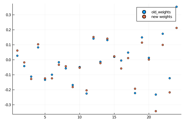

Weights modified according to their gradient.

权重根据其梯度进行修改。

Now to get started. First we’ll import the packages we’ll use. That’s Zygote and a few others we’ll use for plotting and calculating statistics.

现在开始。 首先，我们将导入将使用的软件包。 这就是Zygote和我们将用于绘制和计算统计数据的其他几个。

using Zygote
using Stats
using Plots
using StatsPlots

We’ll need both training data and some matrices to act as neural weights, which the functions below will produce for us.

我们需要训练数据和一些矩阵来充当神经权重，下面的函数将为我们提供这些权重。

get_xor = function(num_samples=512, dim_x=3)
    x = 1*rand(num_samples,dim_x) .> 0.5
    y = zeros(num_samples,1)    for ii = 1:size(y)[1]
        y[ii] = reduce(xor, x[ii,:])
    end    x = x + randn(num_samples,dim_x) / 10    return x, y
endinit_weights = function(dim_in=2, dim_out=1, dim_hid=4)
    wxh = randn(dim_in, dim_hid) / 8
    why = randn(dim_hid, dim_out) / 4
    θ = Dict(:wxh => wxh, :why => why)
    return θ
end

This next bit defines the model we’ll be training: a tiny MLP with 1 hidden layer and no biases. We also need to set up a few helper functions to provide loss and other training metrics (accuracy). To use Zygote’s automatic differentiation capabilities, we need a function that returns a scalar objective function.

接下来的一点定义了我们将要训练的模型：一个微小的MLP，具有1个隐藏层并且没有偏差。 我们还需要设置一些辅助功能来提供损失和其他训练指标(准确性)。 要使用Zygote的自动微分功能，我们需要一个返回标量目标函数的函数。

f(x, θ) = σ(σ(x * θ[:wxh]) * θ[:why])get_accuracy(y, pred, boundary=0.5) = mean(y .== (pred .> boundary))
log_loss = function(y, pred)
    return -(1 / size(y)[1]) .* sum(y .* log.(pred) .+ (1.0 .- y)
             .* log.(1.0 .- pred))endget_loss = function(x, θ, y, l2=6e-4)pred = f(x, θ)
    loss = log_loss(y, pred)
    loss = loss + l2 * (sum(abs.(θ[:wxh].^2))    
           + sum(abs(θ[:why].^2)))
    return lossend

The gradient function from Zygote does as the name suggests. We need to give gradient a function that returns our objective function (log loss in this case), which is why we made an explicit get_loss function earlier. We'll store the results in a dictionary called dθ, and update our model parameters by following gradient descent. The function below defines our training loop.

顾名思义，Zygote的gradient函数可以做到。 我们需要给gradient函数一个返回目标函数的函数(在这种情况下为对数丢失)，这就是为什么我们较早地get_loss了一个明确的get_loss函数的原因。 我们将结果存储在名为dθ的字典中，并通过遵循梯度下降来更新模型参数。 下面的函数定义了我们的训练循环。

train = function(x, θ, y, max_steps=1000, lr=1e-2, l2_reg=1e-4)
    disp_every = max_steps // 100    losses = zeros(max_steps)
    acc = zeros(max_steps)    for step = 1:max_steps
        pred = f(x, θ)
        loss = log_loss(y, pred)
        losses[step] = loss 
        acc[step] = get_accuracy(y, pred)        dθ = gradient((θ) -> get_loss(x, θ, y, l2_reg), θ)        θ[:wxh], θ[:why] = θ[:wxh] .- lr 
                .* dθ[1][:wxh], θ[:why] .- lr .* dθ[1][:why]       
        if mod(step, disp_every) == 0
            val_x, val_y = get_xor(512, size(x)[2]);
            pred = f(val_x, θ) 
            loss = log_loss(val_y, pred)
            accuracy = get_accuracy(val_y, pred)            println("$step loss = $loss, accuracy = $accuracy")
            #save_frame(θ, step);       end    end
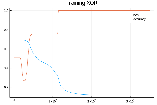
    return θ, losses, accend

With all our functions defined, it’s time to set everything up and start training. We’ll use violin plots from the StatsPlots package to show how the distributions of weights change over time, using a plot function with the ! in-place modifier to add more plots to the current figure. If we want to display more than 1 figure per notebook cell, and we do, we need to explicitly call display on the figure we want to show.

定义好所有功能后，就该进行设置并开始培训了。 我们将使用StatsPlots包中的violin图，使用带有!的plot函数来显示权重的分布随时间的变化! 就地修饰符可向当前图形添加更多图。 如果我们要在每个笔记本单元格中显示多个图形，并且需要这样做，则需要在要display的图形上显式调用display 。

dim_x = 3
dim_h = 4
dim_y = 1
l2_reg = 1e-4
lr = 1e-2
max_steps = 1400000θ = init_weights(dim_x, dim_y, dim_h)
x, y = get_xor(1024, dim_x)println(size(x))plt = violin([" "], reshape(θ[:wxh],dim_x * dim_h), label="wxh", title="Weights", alpha = 0.5)
violin!([" "], reshape(θ[:why],dim_h*dim_y), label="why", alpha = 0.5)
display(plt)θ, losses, acc = train(x, θ, y, max_steps, lr, l2_reg)plt = violin([" "], reshape(θ[:wxh],dim_x * dim_h), label="wxh", title="Weights", alpha = 0.5)
violin!([" "], reshape(θ[:why],dim_h*dim_y), label="why", alpha = 0.5)
display(plt)steps = 1:size(losses)[1]
plt = plot(steps, losses, title="Training XOR", label="loss")
plot!(steps, acc, label="accuracy")
display(plt)

Weights changing over the course of a training, learning curve shown on the right.

权重在训练过程中变化，右侧显示学习曲线。

Finally, it’s a good idea to generate a test set to figure how badly our model is overfitted to the training data. If you’re unlucky and get poor performance from your model, try changing some of the hyperparameters like learning rate or L2 regularization. You can also generate a larger training dataset for better performance, or try changing the size of the hidden layer by changing dim_h. Heck, you could even modify the code to add L1 regularization or add layers to the MLP, so knock your socks off and have a go.

最后，生成一个测试集以判断我们的模型对训练数据的拟合有多严重是一个好主意。 如果您不走运，并且模型效果不佳，请尝试更改一些超参数，例如学习率或L2正则化。 您也可以生成更大的训练数据集以获得更好的性能，或者尝试通过更改dim_h来更改隐藏层的大小。 哎呀，您甚至可以修改代码以添加L1正则化或向MLP添加层，因此请脱颖而出。

test_x, test_y = get_xor(512,3);pred = f(test_x, θ);
test_accuracy = get_accuracy(test_y, pred);
test_loss = log_loss(test_y, pred);println("Test loss and accuracy are $test_loss and $test_accuracy")>>Test loss and accuracy are 0.03354685023541572 and 1.0

测试与验证 (testing vs validation)

The difference between a test and validation dataset is blurry when we generate data on demand as we do here, but normally you wouldn’t want to go back and modify your training algorithm after running your model on a static test dataset. That sort of behavior runs a high risk of data leakage as you can keep tweaking training until you get good performance, but if stop only when the test score is good you’ll actually have settled on a lucky score. That doesn’t tell you anything about how the model will behave with actual test data that it hasn’t seen before, and this happens often in the real world when researchers collectively iterate on a few standard dataset. Of course there will be incremental improvement every year on MNIST if everyone keeps fitting their research strategy to the test set!

当我们按照此处的方法按需生成数据时，测试数据集和验证数据集之间的差异是模糊的，但是通常您不希望在静态测试数据集上运行模型后返回并修改训练算法。 这种行为会带来数据泄露的高风险，因为您可以不断调整训练直到获得良好的性能，但是如果仅在测试成绩良好时停止，您实际上将获得一个幸运的分数。 这并没有告诉您有关该模型如何使用以前从未见过的实际测试数据运行的任何信息，而这通常发生在现实世界中，当研究人员共同迭代几个标准数据集时。 当然，如果每个人都将自己的研究策略与测试集保持一致，那么MNIST每年将得到逐步改进 ！

In any case, thanks for stopping by and I hope you enjoyed exploring automatic differentiation in Julia as I did.

无论如何，感谢您的光临，我希望您像我一样喜欢在Julia中探索自动区分。

翻译自: https://medium.com/sorta-sota/learning-xor-with-julia-and-zygote-16003f171ae0

julia 学习