深度学习技术优化方法比较_深度学习中普遍使用的优化技术

深度学习技术优化方法比较

In this article we will be looking briefly at various optimization techniques widely used in Deep Learning. Before reading this article, if you wanted the mathematical explanation and equation, then this is not for you. This article simply briefs about the various techniques available and the ones that Keras package gives us.

在本文中，我们将简要介绍深度学习中广泛使用的各种优化技术。 在阅读本文之前，如果您需要数学解释和方程式，那么此内容不适合您。 本文仅简要介绍了可用的各种技术以及Keras软件包为我们提供的技术。

In simple words, Optimization algorithms are responsible for reducing losses and provide most accurate results possible. The weight is initialized using some initialization strategies and is updated with each epoch according to the equation. The best results are achieved using some optimization strategies or algorithms called Optimizer.

简而言之，优化算法负责减少损失并提供最准确的结果。 使用一些初始化策略对权重进行初始化，并根据等式在每个时期更新权重。 使用某些称为Optimizer的优化策略或算法可获得最佳结果。

Mind Map of Optimizer

优化器思维导图

Some of the techniques that we will be discussing in this article is-

我们将在本文中讨论的一些技术是-

· Gradient Descent

· 梯度下降

· Stochastic Gradient Descent (SGD)

·随机梯度下降(SGD)

· Mini-Batch Stochastic Gradient Descent (MB — SGD)

·小批量随机梯度下降(MB — SGD)

· SGD with Momentum

·SGD与动量

· Nesterov Accelerated Gradient (NAG)

·Nesterov加速渐变(NAG)

· Adaptive Gradient (AdaGrad)

·自适应渐变(AdaGrad)

· AdaDelta

·AdaDelta

· RMSProp

·RMSProp

· Adam

· 亚当

· Nadam

·那达姆

1.梯度下降 (1. Gradient Descent)

Gradient Descent algorithm

梯度下降算法

A Gradient Descent is an iterative algorithm, that starts from a random point on the function and traverses down its slope in steps until it reaches lowest point of that function. This algorithm is apt for cases where optimal points cannot be found by equating the slope of the function to 0. For the function to reach minimum value, the weights should be altered. With the help of back propagation, loss is transferred from one layer to another and “weights” parameter are also modified depending on loss so that loss can be minimized.

梯度下降是一种迭代算法，它从函数上的随机点开始，然后逐步降低其斜率，直到达到该函数的最低点。 该算法适用于无法通过将函数的斜率等于0来找到最佳点的情况。为了使函数达到最小值，应更改权重。 借助反向传播，损耗会从一层转移到另一层，并且“ weights”参数也将根据损耗进行修改，以便将损耗降至最低。

Cost function: θ=θ−α⋅∇J(θ)

成本函数：θ=θ-α⋅∇J(θ)

As for Gradient Descent algorithm, the entire data set is loaded at a time. This makes it computationally intensive. Another drawback is there are chances the iteration values may get stuck at local minima or saddle point and never converge to minima. To obtain the best solution, the must reach global minima.

至于Gradient Descent算法，则一次加载整个数据集。 这使其计算量大。 另一个缺点是，迭代值可能会卡在局部最小值或鞍点处，而永远不会收敛到最小值。 为了获得最佳解决方案，必须达到全球最低要求。

2. 随机梯度下降(SGD) (2. Stochastic Gradient Descent (SGD))

Stochastic Gradient Descent is an extension of Gradient Descent, where it overcomes some of the disadvantages of Gradient Descent algorithm. SGD tries to overcome the disadvantage of computationally intensive by computing the derivative of one point at a time. Due to this fact, SGD takes more number of iterations compared to GD to reach minimum and also contains some noise when compared to Gradient Descent. As SGD computes derivatives of only 1 point at a time, the time taken to complete one epoch is large compared to Gradient Descent algorithm.

随机梯度下降是梯度下降的扩展，它克服了梯度下降算法的一些缺点。 SGD试图通过一次计算一个点的导数来克服计算量大的缺点。 由于这个事实，与GD相比，SGD需要更多的迭代次数才能达到最小值，并且与Gradient Descent相比还包含一些噪声。 由于SGD一次仅计算1个点的导数，因此与Gradient Descent算法相比，完成一个纪元所花费的时间很大。

3 。 小批量—随机梯度下降 (3. Mini Batch — Stochastic Gradient Descent)

MB-SGD is an extension of SGD algorithm. It overcomes the time-consuming complexity of SGD by taking a batch of points / subset of points from dataset to compute derivative.

MB-SGD是SGD算法的扩展。 它通过从数据集中获取一批点/点子集来计算导数，从而克服了SGD耗时的复杂性。

Note- It is observed that the derivative of loss function of MB-SGD is similar to the loss function of GD after some iterations. But the number iterations to achieve minima in MB-SGD is large compared to GD and is computationally expensive. The update of weights in much noisier because the derivative is not always towards minima.

注意-观察到MB-SGD的损失函数的导数在经过一些迭代后与GD的损失函数相似。 但是，与GD相比，MB-SGD中达到最小值的次数迭代很大，并且计算量很大。 权重的更新要大得多，因为导数并不总是朝向最小值。

In recent times Adaptive Optimization Algorithms are gaining popularity due to their ability to converge swiftly. These algorithms use statistics from previous iterations to speed up the process of convergence.

近年来，自适应优化算法因其快速收敛的能力而越来越受欢迎。 这些算法使用以前迭代的统计信息来加快收敛过程。

在本文的下一部分中，我们将介绍一些自适应优化算法技术。 (In the next segment of the article we will be looking at some Adaptive Optimization Algorithm techniques.)

4. 基于动量的优化器 (4. Momentum based Optimizer)

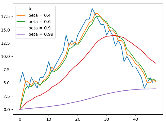
It is an adaptive optimization algorithm which exponentially uses weighted average gradients over previous iterations to stabilize the convergence, resulting in quicker optimization. This is done by adding a fraction (gamma) to the previous iteration values. Essentially the momentum term increase when the gradient points are in the same directions and reduce when gradients fluctuate. As a result, the value of loss function converges faster than expected.

它是一种自适应优化算法，它在先前的迭代中以指数方式使用加权平均梯度来稳定收敛，从而加快了优化速度。 这是通过将分数(gamma)添加到先前的迭代值来完成的。 本质上，当梯度点位于相同方向时，动量项增加，而当梯度波动时，动量项减少。 结果，损失函数的值收敛得比预期的快。

Cost function: V(t)=γV(t−1)+α.∇J(θ)

成本函数：V(t)=γV(t-1)+α.∇J(θ)

θ=θ - V(t)

θ=θ-V(t)

For different values of B, the performance of algorithm is plotted

对于不同的B值，绘制了算法的性能

5. Nesterov加速梯度(NAG) (5. Nesterov Accelerated Gradient (NAG))

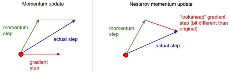
In momentum-based optimization, the current gradient takes the next step based on previous iteration values. But we need a much smarter algorithm that knows when to intuitively stop so that the gradient doesn’t further increase. To do this the algorithm should have an approximate idea of the parameter values in its next iteration. In doing so we can efficiently look ahead by calculating the gradient values wrt to future position of parameters.

在基于动量的优化中，当前梯度将基于先前的迭代值进行下一步。 但是我们需要一个更智能的算法，该算法知道何时直观停止，以免梯度进一步增加。 为此，算法应在其下一次迭代中大致了解参数值。 这样，我们可以通过计算到参数未来位置的梯度值wrt来有效地向前看。

From the previous equation, we know that momentum includes the term [γV(t−1)] to calculate the value of previous iterations. Computing (θ-γV(t−1)) gives us an approximation of next position of parameters[θ]. We can now conclusively look ahead of current parameters by approximating future position with the help of below equation.

从前面的方程式中，我们知道动量包括项[ γV(t-1)]以计算先前迭代的值。 计算( θ-γV(t-1) )给我们近似参数[ θ ]的下一个位置。 现在，我们可以借助下面的公式近似估计未来的位置，最终确定当前的参数。

Cost function: V(t)=γV(t−1)+α.∇J[θ-γV(t−1)]

成本函数：V(t)=γV(t-1)+α.∇J[θ-γV(t-1)]

θ=θ — V(t)

θ=θ— V(t)

By using NAG technique, we are now able to adapt error function with the help of previous and future values and thus eventually speed up the convergence. Now, in the next techniques we will try to adapt alter or vary the individual parameters depending on the importance factor it plays in each case.

通过使用NAG技术，我们现在能够在先前和将来的值的帮助下调整误差函数，从而最终加快收敛速度​​。 现在，在接下来的技术中，我们将尝试根据其在每种情况下发挥的重要作用来更改或更改各个参数。

6. AdaGrad (6. AdaGrad)

Adaptive Gradient as the name suggests adopts the learning rate of parameters by updating it at each iteration depending on the position it is present, i.e- by adapting slower learning rates when features are occurring frequently and adapting higher learning rate when features are infrequent.

顾名思义，自适应梯度通过在每次迭代中根据其存在的位置更新参数来采用参数的学习速率，即-在特征频繁出现时适应较慢的学习速率，而在特征很少发生时适应较高的学习速率。

Technically it acts on learning rate parameter by dividing the learning rate by the square root of gamma, which is the summation of all gradients squared.

从技术上讲，它通过将学习率除以伽马的平方根来影响学习率参数，伽马是所有梯度平方的总和。

In the update rule, AdaGrad modifies the general learning rate N at each step for all the parameters based on past computations. One of the biggest disadvantages is the accumulation of squared gradients in the denominator. Since every added term is positive, the accumulated sum keeps growing during the training. This makes the learning rate to shrink and eventually become small. This method is not very sensitive to master step size and also converges faster.

在更新规则中，AdaGrad根据过去的计算，针对所有参数在每一步中修改通用学习率N。 最大的缺点之一是分母中平方梯度的累积。 由于每个增加的项都是正数，因此在训练期间累积的总和会不断增长。 这使学习率下降，最终变小。 该方法对主步长不是很敏感，并且收敛速度更快。

7. AdaDelta (7. AdaDelta)

It is simply an extension of AdaGrad that seeks to reduce its monotonically decreasing learning rate. Instead of summing all the past gradients, AdaDelta restricts the no. of summation values to a limit (w). In AdaDelta, the sum of past gradients (w) is defined as “Decaying Average of all past squared gradients”. The current average at the iteration then depends only on the previous average and current gradient.

它只是AdaGrad的扩展，旨在降低其单调降低的学习率。 AdaDelta不会限制所有过去的渐变，而不会限制所有的渐变。 求和值的上限为(w)。 在AdaDelta中，过去的梯度之和(w)被定义为“所有过去的平方梯度的衰减平均值”。 然后，迭代时的当前平均值仅取决于先前的平均值和当前梯度。

8. RMSProp (8. RMSProp)

Root Mean Squared Prop is another adaptive learning rate method that tries to improve AdaGrad. Instead of taking cumulative sum of squared gradients like in AdaGrad, we take the exponential moving average. The first step in both AdaGrad and RMSProp is identical. RMSProp simply divides learning rate by an exponentially decaying average.

均方根支撑是另一种尝试提高AdaGrad的自适应学习率方法。 取而代之的是采用指数移动平均值，而不是像AdaGrad那样求平方梯度的累积和。 AdaGrad和RMSProp的第一步是相同的。 RMSProp只是将学习率除以指数衰减的平均值。

9.自适应矩估计(亚当) (9. Adaptive Moment Estimation (Adam))

It is a combination of RMSProp and Momentum. This method computes adaptive learning rate for each parameter. In addition to storing the previous decaying average of squared gradients, it also holds the average of past gradient similar to Momentum. Thus, Adam behaves like a heavy ball with friction which prefers flat minima in error surface.

它是RMSProp和动量的组合。 该方法计算每个参数的自适应学习率。 除了存储平方梯度的先前衰减平均值外，它还保留与动量类似的过去梯度平均值。 因此，亚当的行为就像是一个带有摩擦的沉重的球，它在误差表面上倾向于平坦的最小值。

weight decay update

重量衰减更新

cs231n lecture notes. cs231n讲义 。

10. Nesterov加速自适应矩估计器(Nadam) (10. Nesterov Accelerated Adaptive Moment Estimator (Nadam))

As we have seen in previous section, Adam is a combination of RMSProp and Momentum. Earlier we have also seen that NAG is superior to momentum. Nadam thus incorporates Adam and NAG. To do this we need to modify the momentum term.

正如我们在上一节中所见，Adam是RMSProp和Momentum的组合。 较早之前，我们还看到NAG优于动量。 因此，纳达姆并入了亚当和NAG。 为此，我们需要修改动量项。

source: Nadam paper

资料来源：那当纸

image from

图片来自

Though we have discussed some types of Optimization techniques, not all of these are provided by the popular Keras package.The methods provided by Keras are as listed below-

尽管我们已经讨论了某些类型的优化技术，但并不是所有流行的Keras软件包都提供了这些优化技术。Keras提供的方法如下所示：

SGD

新元

RMSprop

RMSprop

Adam

亚当

Adadelta

阿达达

Adagrad

阿达格勒

Adamax

阿达玛克斯

Nadam

那达姆

Ftrl

Ftrl

To get in detail explanation on how to implement in you Deep Learning model, click on the particular link.

要详细了解如何在您的深度学习模型中实施，请单击特定链接。

Now, that we have had a look at the different optimization techniques, we cannot implement all of them for a same problem. Depending on the case of the problem the approach may change. Now, its your time to decide which optimization technique you want to use in your model.

现在，我们已经研究了不同的优化技术，对于相同的问题，我们无法实现所有优化技术。 根据问题的情况，方法可能会改变。 现在，您就可以决定要在模型中使用哪种优化技术了。

结论 (Conclusion)

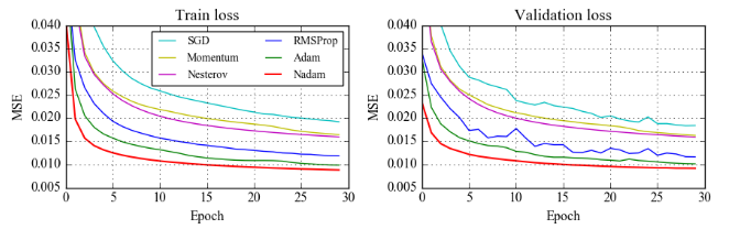
Adam is definitely one of the best optimization algorithms for deep learning and its popularity is growing very fast. While people have noticed some problems with using Adam in certain areas, researches continue to work on solutions to bring Adam results to be on par with SGD with momentum.

亚当绝对是深度学习的最佳优化算法之一，其流行度正在Swift提高。 人们已经注意到在某些领域使用Adam时会遇到一些问题，但研究仍在继续进行，以使Adam的结果与SGD势头相当的解决方案。

翻译自: https://medium.com/@minions.k/optimization-techniques-popularly-used-in-deep-learning-3c219ec8e0cc

深度学习技术优化方法比较