spotify mp3_创建无监督学习的Spotify播放列表

spotify mp3

Spotify presents no shortage of playlists to offer. On my home page right now, I see playlists for: Rap Caviar, Hot Country, Pump Pop, and many others that span all sorts of musical textures.

Spotify会提供很多播放列表。 现在，在我的主页上，我看到以下播放列表：Rap Caviar，Hot Country，Pump Pop和许多其他跨越各种音乐纹理的播放列表。

While many users enjoy going through songs and creating their own playlists based on their own tastes, I wanted to do something different. I used an unsupervised learning technique to find closely related music and create its own playlists.

虽然许多用户喜欢浏览歌曲并根据自己的喜好创建自己的播放列表，但我想做一些不同的事情。 我使用一种无​​监督的学习技术来查找密切相关的音乐并创建自己的播放列表。

The algorithm doesn’t need to classify every song nor does every playlist need to be perfect. Instead, it only needs to produce suggestions I can vet and creatively name, saving me the time of researching songs across different genres.

该算法不需要对每首歌曲进行分类，也不需要对每个播放列表进行完善。 取而代之的是，它只需要提出一些我可以审查和创造性命名的建议，就可以节省研究各种流派的歌曲的时间。

数据集 (The Data Set)

Spotify’s Web API grants developers access to their vast music library. Consequently, data on almost 170,000 songs from 1921 to 2020 were taken and made available on Kaggle. The data spans virtually every genre and features both obscure and popular tracks.

Spotify的Web API允许开发人员访问其庞大的音乐库。 因此，从1921年到2020年，大约有170,000首歌曲的数据被获取并在Kaggle上提供。 数据几乎涵盖了所有流派，并且具有晦涩难懂的流行曲目。

Every song in the data set is broken down by several key musical indicators. Spotify themselves defines each measure, but briefly:

数据集中的每首歌曲都由几个关键的音乐指标细分。 Spotify自己定义了每个度量，但简要说明了：

• Acousticness: how acoustic a song is. Songs with soft pianos and violins score higher while songs with distorted guitars and screaming score lower.
  声音：歌曲的声音。 软钢琴和小提琴的歌曲得分较高，而吉他变形和尖叫的歌曲得分较低。
• Danceability: how appropriate a song is for the dance floor, based on tempo, rhythm stability, beat strength, and overall regularity. Infectious pop songs score higher while stiff classical music scores lower.
  舞蹈性：根据节奏，节奏稳定性，拍子强度和整体规律性，一首歌在舞池中是否合适。 富有感染力的流行歌曲得分较高，而僵硬的古典音乐得分较低。
• Energy: how intense and active a song feels. Hard rock and punk scores higher while piano ballads score lower.
  能量：一首歌有多强烈和活跃。 硬摇滚和朋克得分较高，而钢琴民谣得分较低。
• Instrumentalness: how instrumental a track is. Purely instrumental songs score higher while spoken word and rap songs score lower.
  工具性：轨道的工具性。 纯粹的器乐歌曲得分较高，而口语和说唱歌曲得分较低。
• Liveness: how likely the the song was recorded in front of an audience.
  生动度：这首歌在听众面前录制的可能性。
• Loudness: how loud a track is.
  响度：音轨有多响。
• Speechiness: how vocal a track is. Tracks with no music and only spoken words score higher while instrumental songs score lower.
  语音性：音轨的声音。 没有音乐且只有口语的曲目得分较高，而乐器歌曲的得分较低。
• Valence: how positive or happy a song sounds. Cheerful songs score higher while sad or angry songs score lower.
  价：一首歌听起来有多积极或快乐。 欢快的歌曲得分较高，而悲伤或愤怒的歌曲得分较低。
• Tempo: how fast a song is, in beats per minute (bpm).
  节奏：歌曲的速度，以每分钟的节奏数(bpm)为单位。

清理数据 (Cleaning the Data)

While tempting to dive into analysis, some data cleaning is required. All work will be done in python.

在尝试深入分析时，需要清理一些数据。 所有工作将在python中完成。

import pandas as pd
import numpy as np# read the data
df = pd.read_csv("Spotify_Data.csv")

Before doing anything, the Pandas and NumPy libraries are imported. The final line simply converts the previously saved CSV file to a DataFrame.

在执行任何操作之前，将导入Pandas和NumPy库。 最后一行只是将先前保存的CSV文件转换为DataFrame。

from re import search# Writes function to tell if string is degraded beyond recognition
def is_data_corrupt(string):
    
    # Search for a name with letters and numbers. If no numbers or letters are found, returns None object
    found = search("[0-9A-Za-z]", string)
    
    # Return 1 if corrupt, 0 if not
    return 1 if found == None else 0

At some point during the data collection process, a lot of text became corrupt. As a result, some artists and song names are listed as incomprehensible strings of text, such as “‘周璇’” and “葬花”. As much as I want to know ‘周璇’s greatest hits, I can’t search and compile those values.

在数据收集过程中的某个时刻，许多文本损坏了。 结果，一些艺术家和歌曲名称被列为难以理解的文本字符串，例如“'å'¨ç'‡'”和“è'¬èŠ±”。 我想知道å'¨ç'‡的热门歌曲，但我无法搜索和编译这些值。

To filter corruption, a function called is_data_corrupt() is written that uses regular expressions to check if a string contains numbers, uppercase letters, or lowercase letters. It will mark any string that contains only punctuation or special characters as corrupt, which should find the problematic entries while preserving legitimate song and artist names.

为了过滤损坏，编写了一个名为is_data_corrupt()的函数，该函数使用正则表达式检查字符串是否包含数字，大写字母或小写字母。 它将所有仅包含标点符号或特殊字符的字符串标记为已损坏，这将在保留合法歌曲和歌手姓名的同时找到有问题的条目。

# Create a helper column for artist corruption
df["artists_corrupt"] = df["artists"].apply(lambda x: is_data_corrupt(x))# Create helper column for name corruption
df["name_corrupt"] = df["name"].apply(lambda x: is_data_corrupt(x))# Filter out corrupt artists names
df = df[df["artists_corrupt"] == 0]# Filter out corrupt song names
df = df[df["name_corrupt"] == 0]

After applying the function is_data_corrupt() to both the artists and name columns to create two new, helper columns, any string of text marked as corrupt is filtered out.

在对artist和name列都应用函数is_data_corrupt()以创建两个新的helper列之后，所有标记为已损坏的文本字符串都将被过滤掉。

It’s worth noting that this only marks text that was degraded beyond recognition. Some text still contained partial degradation. For example, famous composer Frédéric Chopin was changed to “Frédéric Chopin”. More extensive data cleaning remedies these entries, but those methods are out of scope for this article.

值得注意的是，这仅标记退化为无法识别的文本。 一些文本仍然包含部分降级。 例如，著名作曲家弗雷德里克·肖邦(FrédéricChopin)被更改为“弗雷德里克·肖邦(FrédéricChopin)”。 更广泛的数据清理可以补救这些条目，但是这些方法不在本文讨论范围之内。

# Gets rid of rows with unspecified artists
df = df[df["artists"] != "['Unspecified']"]

A large share of artists aren’t listed, but instead given the placeholder value “Unspecified”. Since unlisted artists create unnecessary difficulties for finding songs (song titles aren’t unique, after all), these are also filtered.

没有列出大量的艺术家，而是考虑到占位符值为“未指定”。 由于未列出的歌手在查找歌曲时会造成不必要的困难(毕竟歌曲名称不是唯一的)，因此也会对其进行过滤。

# Filter out speeches, comedy routines, poems, etc.
df = df[df["speechiness"] < 0.66]

Finally, purely vocal tracks, such as speeches, comedy specials, and poem readings, present an issue. Because the classifications are based on sound characteristics, these will cluster together.

最后，纯粹的声音轨迹(例如演讲，喜剧特价和诗歌朗诵)提出了一个问题。 因为分类是基于声音特征的，所以它们会聚在一起。

Unfortunately a playlist composed of President Roosevelt’s Fireside Chats and Larry the Cable Guy’s routine makes for a very poor, but amusing, listening experience. Vocal tracks must be categorized on content, which goes beyond the scope of this data.

不幸的是，由罗斯福总统的《炉边闲谈》和有线电视员拉里(Larry the Cable Guy)组成的播放列表会带来非常差但有趣的聆听体验。 声轨必须按内容分类，这超出了此数据的范围。

Consequently, I simply filtered any track with a “speechiness” value of over 0.66. While I may have filtered a few songs, the pay off of removing these tracks is worth it.

因此，我仅过滤了“语音”值超过0.66的任何轨道。 尽管我可能已经过滤了一些歌曲，但删除这些曲目的回报值得。

数据探索 (Data Exploration)

Even before running an unsupervised model, looking for interesting patterns in the data provides insights to how to proceed. All visualizations done with seaborn.

甚至在运行无人监督的模型之前，在数据中寻找有趣的模式还可以洞悉如何进行。 所有可视化均以seaborn完成。

sns.heatmap(df.corr(), cmap = "coolwarm")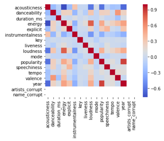

A heat map of all the correlation coefficients in the data. Figure produced by author.

数据中所有相关系数的热图。 图由作者制作。

The above heat map shows how strongly different numerical data correlates. The deep red shows strong positive relationships and the deep blue shows strong negative relationships. Some interesting correlations deserve a few comments.

上面的热图显示了不同数值数据之间的相关程度。 深红色表示强烈的正向关系，深蓝色表示强烈的负向关系。 一些有趣的相关性值得一提。

Unsurprisingly, a strong relationship between popularity and year exists, implying that more recent music is more popular. Between a younger audience who prefers streaming and Spotify actively promoting newer music, this insight confirms domain knowledge.

毫不奇怪，流行度和年份之间存在很强的关系，这意味着更新的音乐更加流行。 在更喜欢流媒体的年轻观众和Spotify积极推广新音乐之间，这种见解证实了领域知识。

In another unsurprising trend, loudness correlates with energy. Intuitively, high energy songs radiate intensity, which often comes with loudness.

在另一个毫不奇怪的趋势中，响度与能量相关。 凭直觉，高能量的歌曲散发出强度，通常伴随响度。

Acousticness shares a few interesting negative relationships. Its inverse relationship with energy and loudness captures the idea of how most people image ballads. Acoustic songs, however, tend to be less popular and their number decreased over time.

声学具有一些有趣的消极关系。 它与能量和响度的反比关系捕捉到了大多数人对民谣的印象。 但是，原声歌曲不太受欢迎，并且随着时间的流逝，其数量减少了。

While surprising given that piano and acoustic guitar tracks stubbornly remain in the public consciousness, this insights says more about the popularity of distortion guitars and synthesizers in music production. Before their advent, every song was considered acoustic and they lost their market share to modernity.

尽管令人惊讶的是，钢琴和原声吉他的音轨一直顽固地存在于公众意识中，但这种见解更多地说明了失真吉他和合成器在音乐制作中的普及。 在他们问世之前，每首歌都被认为是声学的，他们失去了现代性的市场份额。

光学聚类 (OPTICS Clustering)

To create playlists, I used Scikit-Learn’s implementation of OPTICS clustering, which essentially goes through the data to finds areas of high density and assigns them to a cluster. Observations in low density areas aren’t assigned, so not every song will find itself on a playlist.

为了创建播放列表，我使用了Scikit-Learn的OPTICS聚类实现，该聚类实际上是通过数据来查找高密度区域并将它们分配给聚类。 没有分配低密度区域的观测值，因此并非每首歌曲都会在播放列表中显示。

df_features = df.filter([
    "accousticness",
    "danceability",
    "energy",
    "instramentalness",
    "loudness",
    "mode",
    "tempo",
    "popularity",
    "valence"
])

Before running the algorithm, I pulled the columns I wanted to analyze . Most of the features are purely musical based, except popularity, which is kept to help group like artists together.

在运行算法之前，我先列出要分析的列。 除了受欢迎程度以外，大多数功能都是纯粹基于音乐性的，因此可以帮助像艺术家这样的人聚在一起。

Noting that OPTICS clustering uses Euclidean based distance for determining density, not too many columns were added, because high dimensional data skews distance based metrics.

注意到OPTICS聚类使用基于欧几里得距离的距离来确定密度，因此没有添加太多列，因为高维数据会使基于距离的度量倾斜。

from sklearn.preprocessing import StandardScaler# initialize scaler
scaler = StandardScaler()# Scaled features
scaler.fit(df_features)
df_scaled_features = scaler.transform(df_features)

Next the data is changed to a standard scale. While the rest of the features are already normalized between 0 and 1, tempo and loudness use a different scale, which when calculating distances, skews the results. Using the Standard Scaler, everything is brought to the same scale.

接下来，将数据更改为标准比例。 尽管其余功能已经在0和1之间进行了归一化，但速度和响度使用的比例不同，在计算距离时会扭曲结果。 使用Standard Scaler，一切都将达到相同的比例。

# Initialize and run OPTICS
ops_cluster = OPTICS(min_samples = 10)
ops_cluster.fit(df_scaled_features)# Add labels to dataframe
df_sample["clusters"] = ops_cluster.labels_

Finally, OPTICS is run on the data set. Note the parameter min_samples, which denotes the minimum number of observations required to create a cluster. In this case, it dictates the minimum number of songs required to make a playlist.

最后，OPTICS在数据集上运行。 注意参数min_samples，它表示创建聚类所需的最少观察数。 在这种情况下，它规定了制作播放列表所需的最少歌曲数。

Setting min_samples too small will create many playlists with only a few songs, but setting it too high will create a few playlists with a lot of songs. Ten was selected to strike a reasonable balance.

将min_samples设置得太小会创建很多只包含几首歌曲的播放列表，但是将min_samples设置得太高则会创建有很多首歌曲的一些播放列表。 选择十个来达到合理的平衡。

Also note that the data set remains fairly large, so running the algorithm takes time. In my case, my computer worked for a few hours before returning the results.

还要注意，数据集仍然很大，因此运行算法需要时间。 就我而言，我的计算机工作了几个小时才返回结果。

结果 (Outcomes)

As originally stated, I wanted a system to suggest playlists I could manually vet to save myself of the time of researching artists across different genres. Not every songs needed to be classified nor did the play lists need to be perfect.

如最初所述，我想要一个可以建议播放列表的系统，我可以手动对其进行审核，以节省自己研究各种流派的艺术家的时间。 并非所有歌曲都需要分类，播放列表也不需要完善。

Although there’s room for substantial improvement, OPTICS met my expectations. Grouping songs in clusters which followed a general theme, I found a set of interesting playlists that spanned genres I knew nothing about.

尽管仍有很大的改进空间，但OPTICS达到了我的期望。 将歌曲按照一个通用主题进行分组，我发现了一组有趣的播放列表，这些播放列表涵盖了我一无所知的流派。

Unfortunately, most songs weren’t clustered, which means the algorithm lost a large amount of musical diversity. I tried experimenting with different clustering methods (DBSCAN and K-Means), but I received similar results. Quite simply, the data isn’t very dense, so a density-based approach was flawed from the beginning.

不幸的是，大多数歌曲没有聚类，这意味着该算法失去了大量音乐多样性。 我尝试使用不同的聚类方法(DBSCAN和K-Means)进行试验，但收到的结果相似。 很简单，数据不是很密集，因此基于密度的方法从一开始就存在缺陷。

The playlists themselves, however, generally made fun suggestions. While occasionally suggesting bizarre combinations (for example, popular electronic dance music artist Daft Punk found themselves among classical composers), they remained fairly on topic. Consequently, I discovered new artists and learned a lot about music by running this project.

但是，播放列表本身通常提出有趣的建议。 尽管偶尔会提出奇怪的组合(例如，流行的电子舞蹈音乐艺术家Daft Punk发现自己是古典作曲家)，但它们仍然是话题。 因此，我通过运行该项目发现了新的艺术家，并从音乐中学到了很多东西。

That’s the magic of unsupervised learning.

这就是无监督学习的魔力。

播放清单 (The Playlists)

While I could write about different metrics to evaluate the validity of the playlists, I decided there’s no better judge than the crucible of the internet. I lightly edited some of my favorites and encourage anyone to listen and make their own judgement. Note that some songs may contain explicit lyrics.

尽管我可以写出不同的指标来评估播放列表的有效性，但我认为没有比互联网的坩埚更好的判断力了。 我轻轻地编辑了一些我的最爱，并鼓励任何人倾听并做出自己的判断。 请注意，某些歌曲可能包含露骨的歌词。

• Thumping Beats: Tight lyrics and popping baselines in hip hop

  s动的节拍：紧紧的歌词和嘻哈的流行基线

• Synth Candy: A bowl of colorful pop songs

  合成糖：一碗五颜六色的流行歌曲

• Fast n’ Hard: When punk and hard rock hit you in the face

  Fast n'Hard ：当朋克和坚硬的岩石击中你时

• String Section: An evening with violins and cellos

  弦乐部：小提琴和大提琴的夜晚

结论(Conclusions)

While there’s room for improvement, the OPTICS clustering met the requirement and created a diverse set of interesting playlists. Given the issues of density-based approaches, I would revisit this problem with hierarchical clustering, cosine similarity, or some other method to overcome the sparsity in the data.

尽管还有改进的余地，但OPTICS群集满足了要求，并创建了一系列有趣的播放列表。 给定基于密度的方法的问题，我将使用分层聚类，余弦相似性或其他一些克服数据稀疏性的方法来重新探讨这个问题。

More broadly, however, this showcases the power of unsupervised learning in finding patterns which even humans have difficulty quantifying. While not completely automated because it required vetting, using this algorithm showcased how humans and machines can work together to create a more enjoyable end product.

但是，更广泛地讲，这展示了无监督学习在寻找甚至人类都难以量化的模式的能力。 虽然由于需要审查而不能完全自动化，但是使用此算法展示了人与机器如何协同工作以创建更令人愉悦的最终产品。

翻译自: https://towardsdatascience.com/creating-spotify-playlists-with-unsupervised-learning-9391835fbc7f

spotify mp3