


魔方机器人机械部分
Welcome to the second installment of my attempt to solve a Rubik’s Cube via reinforcement learning (RL). Last time, I provided an intro to Markov Decision Processes (MDPs) and formulated the task of solving a Rubik’s Cube as an MDP. If you missed this post or would like a quick refresher, you can check it out here.
欢迎来到我通过强化学习(RL)解决魔方的第二部分。 上次,我向您介绍了马尔可夫决策过程(MDP),并提出了将Rubik's Cube解决为MDP的任务。 如果您错过了这篇文章或想快速回顾一下,可以在此处查看。
At the end of my last post, I left off with a discussion of the Q-function and how we will need to approximate it for our task since the space of state-action pairs is too large. In this post, I will implement a neural network to do exactly that. Along the way, we will explore how the network is trained via the Experience Replay algorithm and provide some initial experimental results. In case you are curious, my actual Python implementation is here. As always, any comments, questions, or feedback is much appreciated!
在上一篇文章的末尾,我结束了对Q函数的讨论,以及由于状态-动作对的空间太大,我们将如何对它进行逼近。 在这篇文章中,我将实现一个神经网络来做到这一点。 在此过程中,我们将探索如何通过“体验重播”算法来训练网络,并提供一些初步的实验结果。 万一您好奇,我的实际Python实现在这里。 与往常一样,任何评论,问题或反馈均深表感谢!
建筑 (Architecture)
Recall that the Q-function takes a state-action pair (s, a) as input and returns a scalar value that roughly represents how “good” it is to take the action a in state s with respect to the ultimate goal of solving the Rubik’s cube. Furthermore, recall that at each solving step, the agent’s strategy will be to take the action which maximizes the Q-function for the current state.
回想一下,Q函数将一个状态-动作对(s,a)作为输入,并返回一个标量值,该标量值大致表示相对于解决以下问题的最终目标,在状态s下采取动作a是“有多好”。魔方。 此外,回想一下,在每个求解步骤中,代理的策略将是采取使当前状态的Q函数最大化的操作。
With these two ideas in mind, we will want to make a neural network that takes some representation of the cube as input and returns a 12 dimensional vector as output. For a given input to the network, s’, each of the 12 output neurons represents the value of the Q-function when taking each of the valid 12 actions in that state. For example, the first neuron could represent Q(s’, Front rotation) and the twelfth neuron could represent Q(s’, Left rotation). Note: the exact mapping between actions and neuron position in the output layer is arbitrary.
考虑到这两个想法,我们将要创建一个神经网络,该神经网络将多维数据集的某种表示形式作为输入,并返回12维向量作为输出。 对于网络的给定输入s' ,当在该状态下采取有效的12个动作中的每个动作时,12个输出神经元中的每个表示Q函数的值。 例如,第一神经元可以代表Q(S',前旋转)和第十二神经元可以代表Q(S',左旋转)。 注意:动作与输出层中神经元位置之间的确切映射是任意的。
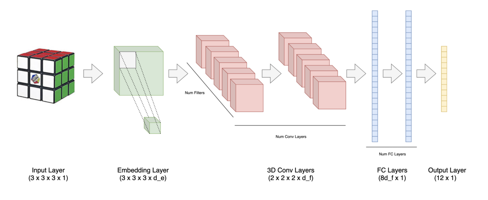
Now that the output has been covered, I will also need a way to represent the Rubik’s Cube state as a numerical input. To accomplish this, we will rely on the concept of embeddings. An embedding is a dense, fixed dimension vector used to represent some object. For example, in NLP, word embeddings are often used to represent individual words and the relationship between two word embedding vectors is meant to capture the semantic relationship between the two corresponding words.
现在已经涵盖了输出,我还将需要一种将Rubik的多维数据集状态表示为数字输入的方法。 为此,我们将依靠嵌入的概念。 嵌入是用于表示某些对象的密集,固定尺寸的向量。 例如,在NLP中,词嵌入通常用于表示单个词,并且两个词嵌入向量之间的关系旨在捕获两个相应词之间的语义关系。
In our case, each of the 27 pieces that makes up a 3x3x3 Rubik’s Cube will have its own unique dₑ dimensional embedding.These embeddings will be learned along with the other weights in the network during training. For implementation details see here.
在我们的案例中,构成3x3x3魔方的27个零件中的每个零件都将具有自己独特的dₑ维嵌入,这些嵌入将在训练过程中与网络中的其他权重一起学习。 有关实现的详细信息,请参见此处。
Between the input layer and the output layer, I have chosen to use a 3D convolutional layer, and then flatten the output from the convolutional layer, and use one more fully connected layer before the 12 dimensional output layer. ELU activations are used on all layers. The rationale behind using ELUs as well as including the convolutional layer are explored in the Initial Results section below.
在输入层和输出层之间,我选择使用3D卷积层,然后对卷积层的输出进行展平,并在12维输出层之前使用一个完全连接的层。 ELU激活可用于所有层。 下面的“初始结果”部分探讨了使用ELU以及包括卷积层的背后原理。
体验重播 (Experience Replay)
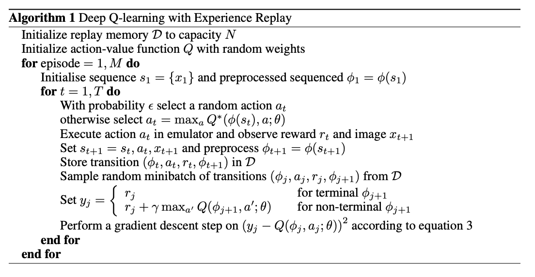
The actual training of the neural network is done via the Experience Replay algorithm. This algorithm is described in the seminal paper on Deep Q-Learning, Playing Atari with Deep Reinforcement Learning by Volodymyr Mnih et al.For the reader’s reference, I have included the pseudo-code from the paper. However, I will try to first describe the procedure at a high level.
神经网络的实际训练是通过“体验重播”算法完成的。 该算法在深Q学习的开创性论文中描述,深层强化学习玩雅达利由弗拉基米尔Mnih等al.For读者的参考,我已经包括了从纸上的伪代码。 但是,我将尝试首先从较高的角度描述该过程。
Experience replay is an iterative algorithm in which the agent attempts to solve the cube many times. During each attempt, the agent starts with a scrambled cube and takes the actions that it thinks are best (according to it current approximation of the Q-function). Every time the agent takes an action, the action, the current state, the resulting state, and an estimate of the action’s “goodness” are all stored as a tuple in something called a replay buffer. The replay buffer is simply a collection of these past “experience” tuples. Mini-batches of these tuples are then sampled from this buffer to make updates to the neural network via gradient descent. Performing updates to the network based on past episodes is a form of off-policy learning. This is in contrast to making updates based on the current episode, which is referred to as on-policy learning (another major branch of RL algorithms).
体验重播是一种迭代算法,代理会尝试多次解决多维数据集。 在每次尝试期间,代理均从一个加扰的多维数据集开始,并采取其认为最佳的操作(根据其对Q函数的当前近似值)。 每次代理执行一个动作时,该动作,当前状态,结果状态以及该动作的“良好”估计都作为元组存储在称为重播缓冲区的内容中。 重播缓冲区只是这些过去的“经验”元组的集合。 然后从该缓冲区中采样这些元组的迷你批,以通过梯度下降对神经网络进行更新。 根据过去的事件对网络执行更新是一种非策略学习的形式。 这与基于当前情节进行更新相反,后者被称为基于策略学习(RL算法的另一个主要分支)。
During the first attempts to solve the cube, the neural network is untrained and so the agent makes nearly random actions to try and solve the cube. However, this series of random actions will eventually lead the agent to solve the cube by chance during one of the episodes. At this point a reward signal will be added to the replay buffer. As the agent keeps training, it will start to include the “experience” tuple that contains this reward signal in the mini-batches used for the gradient descent weight updates. This will slowly improve the Q-function approximation and cause the agent’s actions in subsequent training episode to become a little less random. This will result in further instances of solved cubes and more “good” episodes to be added to the replay buffer. This process is a virtuous cycle and will lead to the agent becoming better at solving the task.
在初次尝试解决多维数据集期间,神经网络未受训练,因此代理会采取几乎随机的动作来尝试解决多维数据集。 但是,这一系列随机动作最终将导致特工在其中一个情节中偶然解决立方体。 此时,奖励信号将添加到重播缓冲区。 随着代理不断训练,它将开始在包含用于梯度下降权重更新的迷你批中包含包含该奖励信号的“体验”元组。 这将缓慢改善Q函数的逼近度,并使代理在后续训练情节中的动作变得随机性降低。 这将导致多维数据集已解决的更多实例,并将更多“好”情节添加到重播缓冲区。 这个过程是一个良性循环,将导致代理更好地解决任务。
However, one thing to note is that sometimes during this process the agent can get stuck in a local minima of sorts. For example, the agent may only know how to solve the cube from certain shuffled states but not others. To try and push the agent out of these local minima, every so often, the agent will take a random action instead of the action prescribed by it’s Q-function approximation. This random action gives the agent a chance to solve the cube in a completely new way and learn something new.
但是,需要注意的一件事是,有时在此过程中,代理可能会陷入局部的最小值中。 例如,代理可能只知道如何从某些混洗状态中解出多维数据集,而不是其他状态。 为了尝试将智能体从这些局部极小值中推出,智能体经常会采取随机动作,而不是Q函数逼近所规定的动作。 这种随机动作使代理有机会以全新的方式解决多维数据集并学习新的知识。
The likelihood of taking this random action is controlled by a parameter epsilon (between 0 and 1), which is why this strategy is usually referred to as an epsilon-greedy strategy. More broadly, within RL, the epsilon-greedy strategy is a method of exploration. Exploration, or discovering new ways to complete the task at hand is often contrasted with exploitation, or leveraging the agent’s existing knowledge to solve the task. These two concepts are often described in terms of a trade-off and are an important component of reinforcement learning.
采取此随机动作的可能性由参数epsilon(介于0和1之间)控制,这就是为什么将此策略通常称为epsilon-greedy策略的原因。 更广泛地说,在RL中, ε贪婪策略是一种探索方法。 探索或发现完成手头任务的新方法通常与开发或利用代理人的现有知识来解决任务形成对照。 这两个概念通常以权衡的方式进行描述,并且是强化学习的重要组成部分。
初步结果 (Initial Results)
For my initial round of experimentation, I started with a very simple set-up with the goal being to help decide the architecture for my Q-function approximation. The task was to solve a Rubik’s Cube that was a shuffle distance of 3 from the solved state. By shuffle distance of 3, I simply mean that starting from a solved cube, three random rotations are applied sequentially to the cube. This shuffled state is the starting point from which the agent attempts to reach the solved state during each episode (the cube is shuffled in a different way before each episode). Furthermore, the agent is limited to at most 5 moves per episode to solve the cube.
在我的第一轮实验中,我从一个非常简单的设置开始,目的是帮助确定我的Q函数逼近的体系结构。 任务是解决距已解决状态3的随机移动距离的魔方。 随机移动距离3是指从一个已解决的多维数据集开始,将三个随机旋转顺序应用于该多维数据集。 此改组状态是代理在每个情节中尝试达到已解决状态的起点(多维数据集在每个情节之前以不同的方式改组)。 此外,代理人每集最多只能执行5步才能解决该问题。
Training was done for 1000 episodes, with the exploration rate, epsilon, starting at 100% and linearly decaying to 10% over the first 100 episode, and after that staying constant at 10%. A replay buffer of size 128 was used, meaning only the last 128 “experience” tuples across all training episodes are stored at a time. Finally, mini-batches of size 16 are used to make the weight updates.
进行了1000次发作的训练,探索率epsilon从100%开始,并在前100次发作中线性衰减至10%,此后保持恒定在10%。 使用了大小为128的重播缓冲区,这意味着一次仅存储所有训练情节中的最后128个“体验”元组。 最后,使用大小为16的迷你批次进行重量更新。
In evaluating the results of these experiments, there are three metrics that I found helpful to track performance:
在评估这些实验的结果时,发现以下三个指标有助于跟踪效果:
Loss (Mean Squared Error): The loss is the squared difference between the network’s current approximation of the Q-value and the observed long run reward for taking a certain action in a given state, averaged over all “experience” tuples in the mini-batch. This loss is in turn averaged over all mini-batches in an episode to get the per-episode loss. As a general rule, the loss should converge as the network learns, with occasional spikes when the agent rethinks its strategy.
损失(均方误差):损失是网络当前对Q值的近似值与在给定状态下采取某种行动所观察到的长期奖励之间的平方差,该平均值是迷你模型中所有“经验”元组的平均值批量。 反过来,将这一损失在一个情节中的所有迷你批处理中平均,以得出每集的损失。 通常,损失应随着网络的学习而收敛,当代理重新考虑其策略时,偶尔会出现峰值。
Validation Accuracy: A more direct approach to evaluating agent performance is to use a hold-out set of shuffled cubes. Specifically, I used a set of 100 cubes with a shuffle distance of 3 and tested the network every 25 episodes of training. The number of cubes from this set that the agent was able to correctly solve in 5 moves or less, divided by 100, is reported as the validation accuracy.
验证准确性:评估代理性能的一种更直接的方法是使用一组拖曳的多维数据集。 具体来说,我使用了一组100个多维数据集,它们的拖曳距离为3,并且每25个训练集测试一次网络。 代理可以在5步或更少的时间内正确解决的多维数据集数量除以100,即报告为验证准确性。
Avg. Max Q Value: The final evaluation metric is taken from the Atari paper. Every 25 episodes, for the same set of cubes used for validation accuracy, the initial shuffled states for each cube are passed through the network and the maximum Q-value over actions is recorded. These maximum Q-values are then averaged together. The rationale for doing this is that as the agent gets smarter, it will have a stronger sense of how a particular action will lead to solving the cube. This means the Q-value for that action (which is the sum of the current reward and all discounted future rewards) will hopefully increase as well. Over training, if the agent is improving, we will therefore expect to see this metric increase.
平均最大Q值:最终评估指标来自Atari论文。 对于用于验证准确性的同一组多维数据集,每隔25集,每个多维数据集的初始混洗状态都会通过网络传递,并记录操作中的最大Q值。 然后将这些最大Q值一起平均。 这样做的理由是,随着代理变得越来越聪明,它将对特定动作如何导致解决多维数据集有更强的认识。 这意味着该操作的Q值(即当前奖励和所有折扣未来奖励的总和)也有望增加。 经过培训后,如果业务代表正在改善,我们将期望看到这一指标增加。
实验1:卷积与全连接层 (Experiment 1: Convolutions vs Fully Connected Layers)
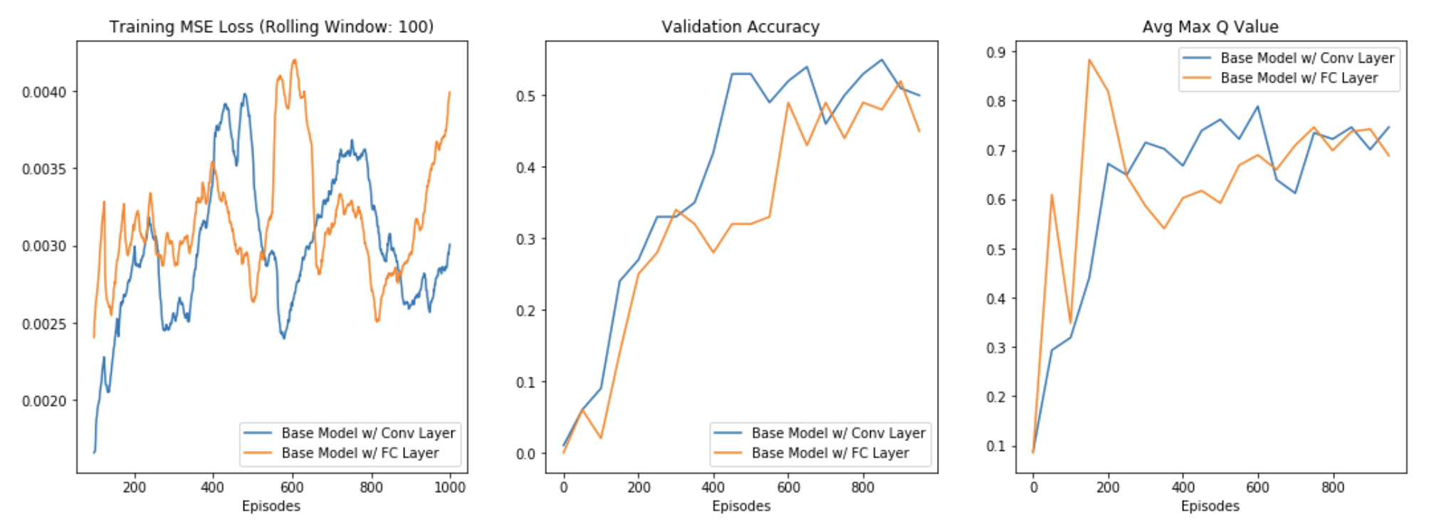
The first experiment was to assess if using convolutional layers was necessary. The alternative being after the embedding layer to simply concatenate all embeddings into a flat (27 * dₑ) dimensional vector. Comparing these two architectures across all three performance metrics, the results are inconclusive with perhaps a slight edge toward using the convolutional layer. The model with a convolutional layer has a slightly higher validation accuracy over training. Furthermore, the average max Q value seems to increase much more smoothly for the model with a convolutional layer. An unfounded hunch tells me this is indicative of a more stable training process.
第一个实验是评估是否需要使用卷积层。 另一种选择是在嵌入层之后,将所有嵌入简单地连接到一个平面(27 * dₑ )尺寸向量中。 在所有三个性能指标上比较这两种体系结构,结果尚不确定,可能在使用卷积层方面略有优势。 具有卷积层的模型具有比训练更高的验证精度。 此外,对于具有卷积层的模型,平均最大Q值似乎更加平滑地增加。 毫无根据的预感告诉我,这表明培训过程更加稳定。
Based more so on the validation accuracy and a prior belief that convolutional layers will work well with the symmetry of the Rubik’s cube, I elected to keep the convolutional layer in my architecture. A perhaps more grounded rationale is also that the convolutional layer has fewer parameters than the fully connected layer (8,020 vs. 67,550).
基于验证准确性以及基于卷积层将与Rubik立方体的对称性很好地结合的先验信念,我选择将卷积层保留在我的体系结构中。 也许更扎根的理由还在于,卷积层的参数少于完全连接的层(8,020 vs. 67,550)。
实验2:ELU与ReLU激活 (Experiment 2: ELU vs ReLU Activation)
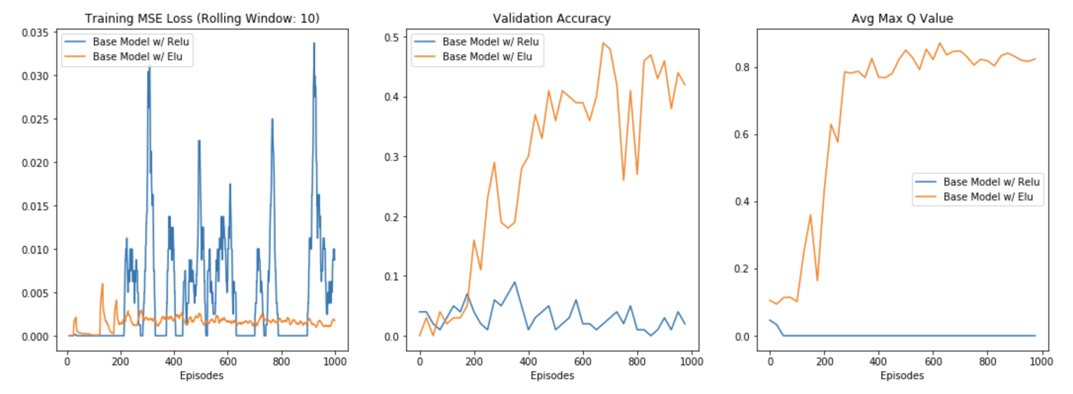
The second experiment I ran was to help choose the activation function for each layer of the neural network. Initially, I had chosen ReLU activations and was noticing some strange behavior. At a shuffle distance of 3, the agent was not learning anything as evidenced by the diverging loss function and the validation accuracy hovering around random chance. The key diagnostic however, was that the average max Q-value was very quickly flatlining to 0 during training.
我进行的第二个实验是帮助选择神经网络每一层的激活函数。 最初,我选择了ReLU激活,并注意到一些奇怪的行为。 在3的混洗距离下,代理没有学习到任何东西,分散的损失函数和验证准确度都徘徊在随机机会上,证明了这一点。 然而,关键的诊断是,在训练期间,平均最大Q值很快就趋于平坦至0。
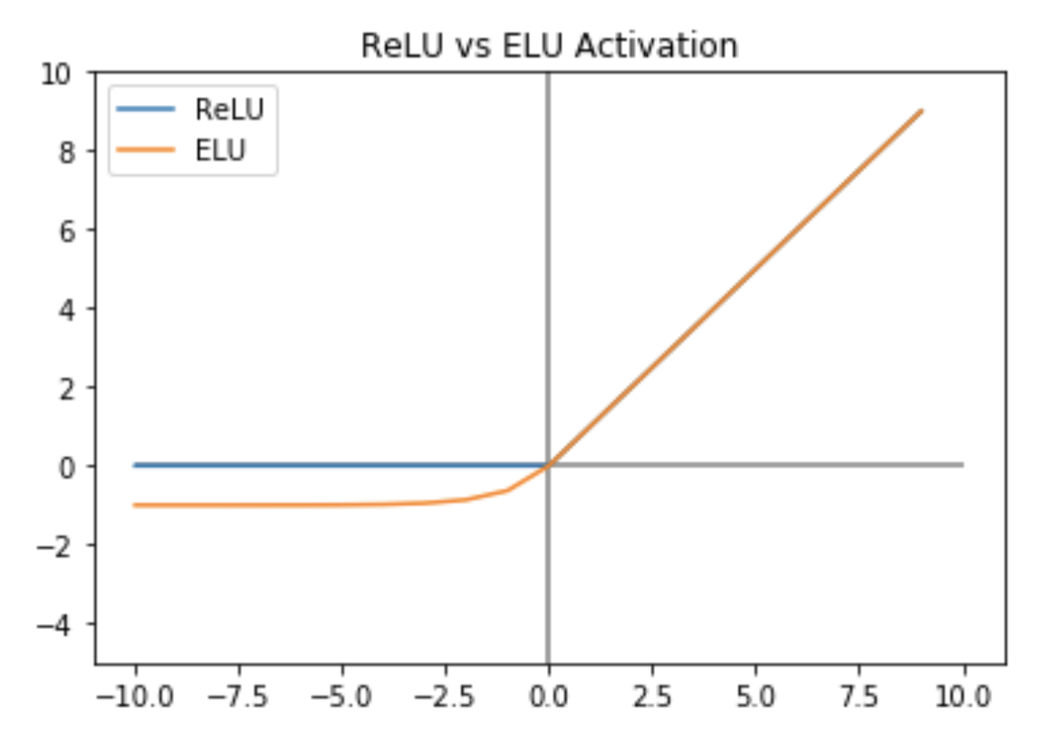
This observation was evidence of a dying ReLU problem. Dying ReLUs occur when the layer proceeding the ReLU activation function produces negative values. For reference, ReLUs are defined to take the constant value of 0 for all negative values. This means that the gradient through the activation will also be 0 during backprop and no weight update will occur. Unless the underlying layer can achieve a positive value at some point later in training, the layer output will always be 0. We see this problem in the graph below, where the average max Q-value (essentially the max value of the output neurons) for the ReLU model is 0.
该观察结果证明了即将死去的ReLU问题。 当进行ReLU激活功能的层产生负值时,将出现垂死的ReLU。 作为参考,ReLU定义为所有负值均取恒定值0。 这意味着在反向传播期间,通过激活的梯度也将为0,并且不会发生权重更新。 除非底层在训练后的某个时刻可以在某个点上获得正值,否则该层的输出将始终为0。我们在下图中看到此问题,其中平均最大Q值(基本上是输出神经元的最大值) ReLU模型的值为0。
Fortunately, this problem can be avoided using an ELU activation function, which maintains a slightly decreasing output for input less than 0. This means that it will have a negative (and non-zero) gradient during backprop, which allows for some gradient flow and prevents the neuron from completely shutting off. When I switched to using ELUs instead of ReLUs, I marked a vast improvement in training across all three evaluation metrics as seen below.
幸运的是,可以使用ELU激活函数避免此问题,该函数为输入小于0的输出保持略有减少的输出。这意味着在反向传播期间它将具有负(非零)梯度,从而允许一些梯度流和防止神经元完全关闭。 当我改用ELU而不是ReLU时,我在所有三个评估指标的训练上都取得了巨大的进步,如下所示。
On the basis of the above experiments, the architecture that I settled on for further experimentation is:
根据以上实验,我确定用于进一步实验的体系结构是:

In my next post, using this architecture as a starting point, I will attempt to increase the shuffle distance of cubes that the agent is able to solve, thereby increasing the complexity of the task. I will also discuss the effects of combining the output of the neural network with a Monte Carlo Search Tree, a common approach in RL and one that is used in the previously mentioned McAleer paper as well.
在我的下一篇文章中,以该体系结构为起点,我将尝试增加代理能够解决的多维数据集的混洗距离,从而增加任务的复杂性。 我还将讨论将神经网络的输出与蒙特卡洛搜索树相结合的效果,蒙特卡洛搜索树是RL中的一种常用方法,并且在前面提到的McAleer论文中也使用了这种方法。
Thank you for reading part two of my Rubik’s Cube series! I hope you found it interesting and would love to discuss any comments or further the conversation in the comments below. Stay tuned for Part 3!
感谢您阅读我的魔方系列的第二部分! 希望您觉得它有趣,并希望在下面的评论中讨论任何评论或进一步讨论。 请继续关注第3部分!
魔方机器人机械部分


 1862
1862

 被折叠的 条评论
为什么被折叠?
被折叠的 条评论
为什么被折叠?
 到【灌水乐园】发言


