揭秘功能工程和基于驾驶员的预测选择

Welcome to the second part of my 3-blog series on creating a robust driver based forecasting engine. The first part gave a brief introduction to time series analysis and gives readers the tools needed to makes sense of time series datasets and cleaning it up (Link here). We will be now looking at the next step in our analysis.

欢迎来到我的3博客系列文章的第二部分，该系列文章是关于创建基于驱动程序的强大预测引擎的。 第一部分简要介绍了时间序列分析，并为读者提供了理解时间序列数据集并进行清理所需的工具(链接此处)。 现在，我们将研究分析的下一步。

While working with one of the leading data analytics teams in India, I have realized that there are two key elements which lead to actionable insights for our clients: Feature Engineering and Feature Selection. Feature engineering refers to the process of creating new variables from existing ones which capture hidden business insights. Feature selection involves making the right choices about which variable to choose for our forecasting models. Both these skills are a combination of art and science which need some practice to perfect.

在与印度领先的数据分析团队之一合作时，我意识到有两个关键要素可为我们的客户带来切实可行的见解： Feature Engineering和Feature Selection 。 功能工程是指从现有变量创建新变量的过程，这些变量捕获隐藏的业务洞察力。 特征选择包括正确选择要为我们的预测模型选择的变量。 这两种技能都是艺术和科学的结合，需要一些实践才能完善。

In this article, we will explore the different types of features which are commonly engineered during forecasting projects and the rationale for using them. We will also look at a comprehensive set of methods that we can use to select the best features and a handy method to combine all the these methods. To dig deeper on feature analysis, one can refer to the book “Feature Engineering and Selection: A Practical Approach for Predictive Models” by Max Kuhn and Kjell Johnson

在本文中，我们将探讨在预测项目期间通常设计的不同类型的功能以及使用这些功能的原理。 我们还将研究一套全面的方法，可用于选择最佳功能，以及一种方便的方法来组合所有这些方法。 要深入研究特征分析，可以参考Max Kuhn和Kjell Johnson撰写的《特征工程与选择：一种预测模型的实用方法》一书。

指数： (Index:)

• Feature Engineering (Lags, Periodic difference, Flags for events etc.)
  特征工程(滞后，周期性差异，事件标志等)
• Feature Selection Methods (Correlation, Lasso Regression, Recursive Feature Selection,Random Forest, Beta Coefficients)
  特征选择方法(相关性，套索回归，递归特征选择，随机森林，Beta系数)
• Combining Feature Selection Methods
  组合特征选择方法
• Final words
  最后的话

特征工程(Feature Engineering)

It is common practice to use different ways to represent data fields in a model, and usually some of these representations are better than others. This is the basic idea behind feature engineering — the process of creating representations of data that increase the effectiveness of a model. We will be discussing some of the tried and tested features created from a multivariate time series data and the rationale behind each of them. The dataset being used here is the same as the previous blog in this series. It is a daily dataset on Hong Kong flat prices along with 12 macro economics variables.

通常的做法是使用不同的方式来表示模型中的数据字段，通常这些表示中的某些比其他的要好。 这是要素工程背后的基本思想-创建可增强模型有效性的数据表示的过程。 我们将讨论根据多元时间序列数据创建的一些经过试验和测试的功能，以及每个功能背后的原理。 这里使用的数据集与本系列中的上一个博客相同。 它是有关香港统一价格以及12个宏观经济学变量的每日数据集。

Feature 1: Lags

特征1：滞后

Lag features are values at prior time steps. For example lag 1 of a variable at time t is its value from last period, t-1. As the name suggests, the hypothesis here is that the features have a lagged impact on the target variable. The best way to find the optimal number of lags to chose for each field is to look at cross correlation graphs.Cross correlation graphs show the correlation between the target variable (here, private domestic price index of flats) with various lags of raw features (sales, money supply, etc.).

滞后特征是先前时间步长的值。 例如，变量在时间t的滞后1是其从上一周期t-1开始的值。 顾名思义，这里的假设是要素对目标变量的影响滞后。 找到为每个字段选择的最佳滞后次数的最佳方法是查看互相关图。 互相关图显示了目标变量(这里是公寓的私人国内价格指数)与各种原始特征(销售，货币供应等)之间的相关性。

# Check Optimal Number of Lags
for i in range(3,12):
    pyplot.figure(i, figsize=(15,2)) # add this statement before your plot
    pyplot.xcorr(df.iloc[:,2],df.iloc[:,i],maxlags=45, usevlines=1)
    pyplot.title('Cross Correlation Between Private Domestic (Price Index) and '+ df.columns[i])
    pyplot.show()

• There is a high level of correlation for a large number of lags between the target variable and most of the features.
  对于目标变量和大多数特征之间的大量滞后，存在高度的相关性。
• For this exercise we created 3 lags for each column with the ‘shift’ function as shown below. Ideally, we should add lags till the point where cross correlation drastically drop.
  在本练习中，我们使用“移位”功能为每列创建了3个滞后，如下所示。 理想情况下，我们应该增加延迟直到互相关急剧下降的点。

#Add Lags
predictors2 = predictors1.shift(1)
predictors2 = predictors2.add_suffix('_Lag1')
predictors3 = predictors1.shift(2)
predictors3 = predictors3.add_suffix('_Lag2')
predictors4 = predictors1.shift(3)
predictors4 = predictors4.add_suffix('_Lag3')

Feature 2: Periodic Difference

特征2：周期性差异

This feature is calculated as the difference between the current value of the variable and its previous value. The expectation is that the change in a variable has a stronger relationship than the raw variable itself. We can calculate the periodic difference using the ‘diff’ function (as shown below).

此功能的计算方式是变量的当前值与其先前值之间的差。 期望变量的变化比原始变量本身具有更强的关系。 我们可以使用'diff'函数计算周期差(如下所示)。

#Add Periodic Difference
predictors5 = predictors1.diff()
predictors5 = predictors5.add_suffix('_Diff')

Similarly, one can also calculate month-on-month, year-on-year or quarter-on-quarter changes given the business problems.

同样，鉴于业务问题，还可以计算按月，按年或按季度变化。

Feature 3: Flags for events

功能3：事件标志

Sometimes highlighting key events like holidays helps the model predict better. For example, if we are trying to predict garment sales then a flag for holidays like Christmas, Thanksgiving etc usually help the model predict the sudden peaks during such times better. In our case, we created flags for holidays using the ‘calendar’ function.

有时突出显示关键事件(例如假期)有助于模型更好地进行预测。 例如，如果我们要预测服装的销售量，那么圣诞节，感恩节等假期的旗帜通常可以帮助模型更好地预测这种时期的突然高峰。 在我们的案例中，我们使用“日历”功能创建了假期标记。

# Create Holiday Flagdf['Date'] = pd.to_datetime(df['Date'])
cal = calendar()
holidays = cal.holidays(start=df['Date'].min(), end=df['Date'].max())
df['holidays'] = pd.np.where(df['Date'].dt.date.isin(holidays), 1, 0)
df.head(5)

• To create a flag for events, it is important to have a date column which is in the correct date-time format (example : “YYYY-MM-DD”)
  要为事件创建标志，重要的是要有一个日期列，其日期和时间格式必须正确(例如：“ YYYY-MM-DD”)
• We create a separate list of dates for holidays and for all the values in the date column in our dataset which has a match with this list, we flag it as a holiday
  我们为假期创建了一个单独的日期列表，并为数据集中与该列表匹配的日期列中的所有值创建了一个日期列表，并将其标记为假期

Apart from these common features, based on business context we should try to create additional features which have a strong relationship with the target variable. For example, we created a new feature ‘First Hand Price’ as the ratio between ‘First Hand sales amount’ and ‘First Hand quantity’.

除了这些通用功能之外，我们还应基于业务上下文尝试创建与目标变量有密切关系的其他功能。 例如，我们创建了一个新功能“第一手价格”作为“第一手销售量”与“第一手数量”之间的比率。

#Create a new feature =  First hand price
df['First hand sales price'] = df['First hand sales amount']/df['First hand sales quantity']
predictors1 = df.drop(columns=['Date','Private Domestic (Price Index)','holidays','First hand sales amount','First hand sales quantity'],axis=1) # Add  if applicable
predictors1.head(5)

Feature 4: Financial data

功能4：财务数据

It is very easy to download financial data like stock prices and indexes in Python. There are many options out there (Quandl, Intrinion, AlphaVantage, Tiingo, IEX Cloud, etc.), however, Yahoo Finance is considered the most popular as it is the easiest one to access (free and no registration required). Although we do not use it in our exercise but I have added the relevant pieces of code needed to extract the following:

在Python中下载股票价格和指数等财务数据非常容易。 那里有很多选项(Quandl，Intrinion，AlphaVantage，Tiingo，IEX Cloud等)，但是，Yahoo Finance被认为是最受欢迎的，因为它是最容易访问的一种(免费且无需注册)。 尽管我们不在练习中使用它，但是我添加了提取以下内容所需的相关代码：

1. Stock Price of a company:
   公司股票价格：

#### Additional features: Stock Price
import yfinance as yf
from yahoofinancials import YahooFinancialsyahoo_financials = YahooFinancials('CRM')stock_price = yahoo_financials.get_historical_price_data(start_date='2018-08-01', 
                                                  end_date='2020-08-01', 
                                                  time_interval='monthly')stock_price_df = pd.DataFrame(stock_price['CRM']['prices'])
stock_price_df = stock_price_df.drop('date', axis=1).set_index('formatted_date')
stock_price_df = pd.DataFrame(stock_price_df['close'])
stock_price_df.columns = ['Stock_Price']stock_price_df

2. Stock price index of the competitors of a company

2.公司竞争对手的股价指数

# Additional features:  Stock Price Index from multiple companiesscaler = StandardScaler()
# transform x data
scaled_stock = scaler.fit_transform(stock_price_df_c)
column_name = competitor_stock[i]
stock_price_df_comp[column_name] = scaled_stock[:,0]
                    
col = stock_price_df_comp.loc[: , "ADBE":"ORCL"]
stock_price_df_comp['Competitor_Stock_Index'] = col.mean(axis=1)
stock_price_df_comp = pd.DataFrame(stock_price_df_comp['Competitor_Stock_Index'])stock_price_df_comp

3. S&P 500

3.标普500

#Additional features:  S&P 500import datetimepd.core.common.is_list_like = pd.api.types.is_list_likeimport pandas_datareader.data as webstart = datetime.datetime(2018, 8, 1)
end = datetime.datetime(2020, 8, 1)SP500 = web.DataReader(['sp500'], 'fred', start, end)SP500_df = SP500.resample('MS').mean()SP500_df

特征选择方法 (Feature Selection Methods)

Feature selection is a critical step for most data science projects as it enables the models to train faster, reduces the complexity and makes it easier to interpret. It has the potential to improve model performance and reduce the problem of overfitting if the optimal set of features are chosen. We will be discussing various methods and their respectives rules for selecting the best features.

对于大多数数据科学项目而言，特征选择是至关重要的一步，因为它使模型能够更快地训练，降低复杂性并使其更易于解释。 如果选择了最佳的特征集，它有可能提高模型性能并减少过度拟合的问题。 我们将讨论选择最佳功能的各种方法及其各自的规则。

Method 1: Variable Importance from Random Forest

方法1：来自随机森林的变量重要性

Random forests consist of multiple decision trees, each of them built over a random sample of the observations from the dataset and a random sample of the features. This random selection guarantees that the trees are not correlated and therefore less susceptible to over-fitting. For forecasting exercises, we use variable importance feature of random forest which measures how much the accuracy decreases when a variable is excluded. To learn more about random forest and variable importance, please refer to this detailed blog by Niklas Donges.

随机森林由多个决策树组成，每个决策树都建立在数据集中观测值的随机样本和要素的随机样本之上。 这种随机选择保证了树木没有相关性，因此不太适合过度拟合。 对于预测演习，我们使用随机森林的变量重要性特征，该特征度量了排除变量后准确性降低了多少。 要了解有关随机森林和变量重要性的更多信息，请参阅Niklas Donges撰写的详细博客。

#1.Select the top n features based on feature importance from random forestnp.random.seed(10)# define the model
model = RandomForestRegressor(random_state = random.seed(10))
# fit the model
model.fit(predictors, Target)# get importance
features = predictors
importances = model.feature_importances_
indices = np.argsort(importances)feat_importances = pd.Series(model.feature_importances_, index=predictors.columns)
feat_importances.nlargest(30).plot(kind='barh')

• We first fit the random forest model and then extract the variable importance.
  我们首先拟合随机森林模型，然后提取变量重要性。

#Final Features from Random Forest (Select Features with highest feature importance)
rf_top_features = pd.DataFrame(feat_importances.nlargest(7)).axes[0].tolist()

• We check the feature importance plot for top 30 variables based on variable importance. We can see that 2 period lag of ‘M3 (HK$ million)’ is the most important feature and after the 7th feature the variable importance falls. So we chose 7 features for this analysis.
  我们根据变量重要性检查前30个变量的特征重要性图。 我们可以看到，最重要的特征是“ M3(百万港元)”两个时期的滞后，而在第七个特征之后，可变的重要性下降了。 因此，我们选择了7个功能进行此分析。

We can optimise the random forest model by tuning the parameters in case the features selected by the default model are not satisfactory. This is an example of embedded method which work by evaluating a subset of features using a machine learning algorithm that employs a search strategy to look through the space of possible feature subsets, evaluating each subset based on the quality of the performance of a given algorithm.

如果默认模型选择的功能不令人满意，我们可以通过调整参数来优化随机森林模型。 这是嵌入式方法的一个示例，该方法通过使用机器学习算法评估要素的子集来工作，该机器学习算法采用搜索策略来浏览可能的要素子集的空间，并根据给定算法的性能来评估每个子集。

Method 2: Pearson Correlation

方法2：皮尔逊相关

We try to find the highly correlated features using the absolute value of pearson correlation. This is an example of a filter method where features are selected on the basis of their scores in various statistical tests.

我们尝试使用皮尔逊相关性的绝对值找到高度相关的特征。 这是过滤方法的一个示例，其中在各种统计测试中根据特征的分数选择特征。

#2.Select the top n features based on absolute correlation with target variable
corr_data1 = pd.concat([Target,predictors],axis = 1)
corr_data = corr_data1.corr()
corr_data = corr_data.iloc[: , [0]]
corr_data.columns.values[0] = "Correlation"
corr_data = corr_data.iloc[corr_data.Correlation.abs().argsort()] 
corr_data = corr_data[corr_data['Correlation'].notna()]
corr_data = corr_data.loc[corr_data['Correlation'] != 1]
corr_data.tail(20)

• We calculate the correlation of each feature with the target variable and sort the features by the absolute values of their correlation.
  我们计算每个特征与目标变量的相关性，并按其相关性的绝对值对特征进行排序。

# Select Features with greater than 90% absolute correlation
corr_data2 = corr_data.loc[corr_data['Correlation'].abs() > .9]
corr_top_features = corr_data2.axes[0].tolist()

• We select the 12 features with greater than 90% absolute correlation. Based on the business context the threshold can be modified.
  我们选择绝对相关度大于90％的12个特征。 根据业务环境，可以修改阈值。

Method 3: L1 regularisation using Lasso regression

方法3：使用Lasso回归进行L1正则化

Lasso or L1 regularisation is based on the property that is able to shrink some of the coefficients in a linear regression to zero. Therefore, such features can be removed from the model. This is another example of an embedded method of feature selection.

套索或L1正则化基于能够将线性回归中的某些系数缩小为零的属性。 因此，可以从模型中删除此类功能。 这是嵌入的特征选择方法的另一个示例。

#3.Select the features identified by Lasso regressionnp.random.seed(10)estimator = LassoCV(cv=5, normalize = True)sfm = SelectFromModel(estimator, prefit=False, norm_order=1, max_features=None)sfm.fit(predictors, Target)feature_idx = sfm.get_support()
Lasso_features = predictors.columns[feature_idx].tolist()
Lasso_features

• We specify the Lasso Regression model and then use the ‘selectFromModel’ function, which will select in theory the features which coefficients are non-zero
  我们指定套索回归模型，然后使用“ selectFromModel”函数，该函数将在理论上选择系数为非零的特征

To learn more about feature selection using Lasso Regression, please refer to this paper by Valeria Fonti.

要了解有关使用套索回归的特征选择的更多信息，请参阅Valeria Fonti的本文。

Method 4: Recursive Feature Selection (RFE)

方法4：递归特征选择(RFE)

RFE is a greedy optimization algorithm which repeatedly creates models and separates out the best or the worst performing feature at each iteration. It constructs the next model with the remaining features until all the features have been used. It finally ranks the features based on the order of their elimination.

RFE是一种贪婪的优化算法，它会反复创建模型，并在每次迭代时分离出性能最佳或最差的功能。 它将使用其余功能构造下一个模型，直到使用完所有功能。 最后，根据特征消除的顺序对特征进行排序。

#4.Perform recursive feature selection and use cross validation to identify the best number of features#Feature ranking with recursive feature elimination and cross-validated selection of the best number of featuresrfe_selector = RFE(estimator=LinearRegression(), n_features_to_select= 7, step=10, verbose=5)
rfe_selector.fit(predictors, Target)
rfe_support = rfe_selector.get_support()
rfe_feature = predictors.loc[:,rfe_support].columns.tolist()
rfe_feature

We use linear regression to perform the recursive feature selection and select top 7 ranked fields. This is a wrapper method of feature selection that attempts to find the “optimal” feature subset by iteratively selecting features based on the model performance.

我们使用线性回归来执行递归特征选择，并选择排名前7位的字段。 这是一种特征选择的包装方法，该方法通过基于模型性能反复选择特征来尝试查找“最佳”特征子集。

Method 5: Beta Coefficients

方法5：Beta系数

The absolute value of the coefficients of a standardized regression, also known as beta coefficients, can be considered a proxy for feature importance. This is a type of filter method of feature selection.

标准化回归系数的绝对值(也称为β系数)可以视为特征重要性的代理。 这是特征选择的一种过滤方法。

#5.Select the top n features based on absolute value of beta coefficients of features# define standard scaler
scaler = StandardScaler()
# transform x data
scaled_predictors = scaler.fit_transform(predictors)
scaled_Target = scaler.fit_transform(Target)sr_reg = LinearRegression(fit_intercept = False).fit(scaled_predictors, scaled_Target)
coef_table = pd.DataFrame(list(predictors.columns)).copy()
coef_table.insert(len(coef_table.columns),"Coefs",sr_reg.coef_.transpose())
coef_table = coef_table.iloc[coef_table.Coefs.abs().argsort()]sr_data2 = coef_table.tail(10)
sr_top_features = sr_data2.iloc[:,0].tolist()
sr_top_features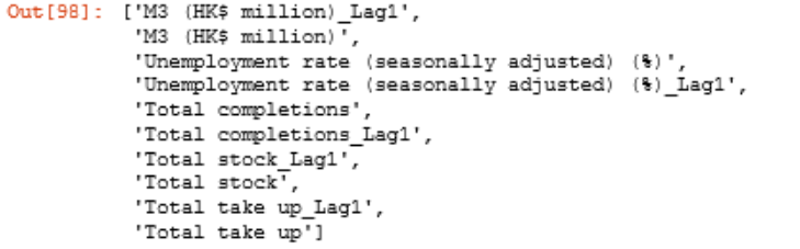

• We standardise the dataset and run a standardized regression with all the features included in it.
  我们对数据集进行标准化，并使用其中包含的所有功能进行标准化回归。
• We select 10 features based on the highest absolute value of beta coefficients.
  我们根据Beta系数的最高绝对值选择10个特征。

组合特征选择方法 (Combining Feature Selection Methods)

Each of these models are good at capturing a particular type of relationship between the features and target variable. For example, beta coefficients are good at identifying the linear relationships while random forest is suitable for spotting non-linear bonds. Based on my experience, I found that trying to combine the results from multiple methods led to more robust results. We will look at one of the ways to do so in this section.

这些模型中的每一个都擅长捕获要素和目标变量之间的特定类型的关系。 例如，β系数擅长于识别线性关系，而随机森林则适合于发现非线性键。 根据我的经验，我发现尝试合并多种方法的结果会得到更可靠的结果。 我们将在本节中探讨实现此目标的方法之一。

# Combining features from all the modelscombined_feature_list = sr_top_features + Lasso_features + corr_top_features + rf_top_featurescombined_feature = {x:combined_feature_list.count(x) for x in combined_feature_list}
combined_feature_data = pd.DataFrame.from_dict(combined_feature,orient='index')combined_feature_data.rename(columns={ combined_feature_data.columns[0]: "number_of_models" }, inplace = True)combined_feature_data = combined_feature_data.sort_values(['number_of_models'], ascending=[False])combined_feature_data.head(100)

• We combine the list of features from each model into one and then check the number of times each feature appears in that list. This indicates the number of methods/models in which the features were selected.
  我们将每个模型的功能列表组合为一个，然后检查每个功能出现在该列表中的次数。 这表明选择特征的方法/模型的数量。
• We select the features which were chosen in majority of the methods. In our case we have 5 models and hence, we picked 3 features which were selected in at least 3 out of 5 methods.
  我们选择大多数方法中选择的功能。 在我们的案例中，我们有5个模型，因此，我们选择了3种特征，这些特征是从5种方法中的至少3种中选择的。

#Final Features: features which were selected in atleast 3 modelscombined_feature_data = combined_feature_data.loc[combined_feature_data['number_of_models'] > 2]
final_features = combined_feature_data.axes[0].tolist()
final_features

The benefit of using this approach to combine feature selection methods is the flexibility to add/remove models as per the business problem at hand. Markov blanket from a bayesian network, forward/backward regression and feature importance from XGBoost are some additional methods on feature selection which can be considered.

使用这种方法组合特征选择方法的好处是可以根据当前的业务问题灵活地添加/删除模型。 贝叶斯网络的马尔可夫毯，向前/向后回归以及XGBoost的特征重要性是可以考虑的一些其他特征选择方法。

最后的话 (Final Words)

With this said Part 2 of the 3-part blog series comes to an end. The readers should now be able to extract various relevant features out of datasets which are relevant for most forecasting exercises. They can also add relevant 3rd party datasets like holiday flags and financial indexes as new features to supplement the raw dataset. Apart from engineering these features, the readers now have an extensive toolkit for selecting the best features based on multiple methods. I would like to again highlight here that feature engineering and selection is combination of art and science. One becomes better at it with experience. The code for the entire analysis can be found here.

这样，由3部分组成的博客系列的第2部分结束了。 读者现在应该能够从与大多数预测活动相关的数据集中提取各种相关特征。 他们还可以添加相关的第三方数据集(如节日标志和财务指标)作为新功能来补充原始数据集。 除了对这些功能进行工程设计之外，读者现在拥有了一个广泛的工具包，可以根据多种方法选择最佳功能。 我想再次强调一下，特征工程和选择是艺术与科学的结合。 随着经验的积累，人们会变得更好。 整个分析的代码可以在这里找到。

Do read the final part of this series where we create an extensive pipeline of tried and tested forecasting models by combining time series and machine learning techniques.

请阅读本系列的最后一部分，在本文中，我们将时间序列和机器学习技术相结合，创建了一系列经过验证的预测模型。

Do you have any questions or suggestions about this blog? Please feel free to drop in a note.

您对此博客有任何疑问或建议吗？ 请随时添加便条。

感谢您的阅读！ (Thank you for reading!)

If you are, like me, passionate about AI, Data Science, or Economics, please feel free to add me on LinkedIn.

如果您像我一样对AI，数据科学或经济学充满热情，请随时在LinkedIn上加我。

翻译自: https://medium.com/@indraneeldb1993ds/demystifying-feature-engineering-and-selection-for-driver-based-forecasting-50ba9b5a0fbc