解释kaggle住房价格，要素工程和岭回归

最新推荐文章于 2022-11-25 11:27:11 发布

weixin_26750481

最新推荐文章于 2022-11-25 11:27:11 发布

阅读量455

点赞数

文章标签： python 机器学习 leetcode

原文链接：https://medium.com/swlh/explained-kaggle-housing-prices-feature-engineering-and-ridge-regression-88934ad37edc

版权

This blog is based on the notebook I used to submit predictions for Kaggle In-Class Housing Prices Competition. My submission ranked 293 on the score board, although the focus of this blog is not how to get a high score but to help beginners develop intuition for Machine Learning regression techniques and feature engineering. I am a final year mechanical engineering student, I started learning python in January 2020 with no intentions to learn data science. Thus, any suggestions in the comments for improvement will be appreciated.

该博客基于我用来提交Kaggle房内价格竞赛的笔记本的笔记本。 我的提交在计分板上排名293，尽管该博客的重点不是如何获得高分，而是帮助初学者发展机器学习回归技术和特征工程的直觉。 我是机械工程专业的大一学生，我从2020年1月开始学习python，无意学习数据科学。 因此，将对评论中的任何改进建议表示赞赏。

介绍 (Introduction)

The scope of this blog is on the data pre-processing, feature engineering, multivariate analysis using Lasso Regression and predicting sale prices using cross validated Ridge Regression.

该博客的范围涉及数据预处理，特征工程，使用Lasso回归的多元分析以及使用经过交叉验证的Ridge回归预测销售价格。

The original notebook also contains code on predicting prices using a blended model of Ridge, Support Vector Regression and XG-Boost Regression, which would make this blog verbose. To keep this blog succinct, code blocks are pasted as images where necessary.

原始笔记本还包含使用Ridge，支持向量回归和XG-Boost回归的混合模型预测价格的代码，这会使该博客变得冗长。为了使本博客简洁，在必要时将代码块粘贴为图像。

The notebook is uploaded on the competition dashboard if reference or code is required : https://www.kaggle.com/devarshraval/top-2-feature-selection-ridge-regression

如果需要参考或代码，则将笔记本上传到比赛仪表板上： https : //www.kaggle.com/devarshraval/top-2-feature-selection-ridge-regression

This data set is of particular importance to novices like me in the sense of the vast range of features. There are a total of 79 features(excluding Id) which are said to explain the sale price of the house, it tests the industriousness of the learner in handling these many features.

就广泛的功能而言，该数据集对像我这样的新手尤为重要。据说共有79个功能(不包括ID)可以解释房屋的售价，它测试了学习者在处理这些功能时的勤奋性。

1.探索性数据分析 (1. Exploratory data analysis)

The first step in any data science project should be getting to know the data variables and target. This stage can make one quite pensive or other hand feel enervated depending on one’s interests. Exploring the data gives an understanding of the problem and feature engineering ideas.

任何数据科学项目的第一步都应该是了解数据变量和目标。这个阶段可以使一个人的沉思或另一只手感到精力充沛，这取决于一个人的兴趣。探索数据可以使您对问题有所了解，并具有功能工程学思想。

It is recommended to read the feature description text file to understand feature names and categorize the variables into groups such as Space-related features, Basement features, Amenities, Year built and remod, Garage features, and etc based on subjective views.

建议阅读特征描述文本文件以了解特征名称，并根据主观观点将变量归类为与空间相关的特征，地下室特征，便利设施，建造年份和改建年份，车库特征等。

This categorization and feature importance becomes more intuitive after a few commands in the notebook such as:

在笔记本中执行以下命令后，此分类和功能重要性将变得更加直观：

corrmat=df_train.corr()
corrmat['SalePrice'].sort_values(ascending=False).head(10)

SalePrice 1.000000OverallQual 0.790982GrLivArea 0.708624GarageCars 0.640409GarageArea 0.623431TotalBsmtSF 0.6135811stFlrSF 0.605852FullBath 0.560664TotRmsAbvGrd 0.533723YearBuilt 0.522897

销售价格1.000000总体质量0.790982格鲁夫区域0.708624车库汽车0.640409车库面积0.623431总计BsmtSF 0.6135811stFlrSF 0.605852FullBath 0.560664TotRmsAbvGrd 0。533723年建成0.522897

Naturally, overall quality of the house is strongly correlated with the price. However, it is not defined how this measure was calculated. Other features closely related are space considerations (Gr Liv Area, Total Basement area, Garage area) and how old the house is (Year Built).

自然，房屋的整体质量与价格密切相关。但是，尚未定义如何计算此度量。与空间息息相关的其他功能还包括空间因素(Gr Liv面积，地下室总面积，车库面积)和房屋的年限(建成年份)。

The correlations give an univariate idea of important features. Thus, we can plot all of these features and remove outliers or multicollinearity. Outliers can skew regression models sharply and multicollinearity can undermine importance of a feature for our model.

相关性给出了重要特征的单变量概念。因此，我们可以绘制所有这些特征并去除异常值或多重共线性。离群值会严重扭曲回归模型，而多重共线性会破坏特征对我们模型的重要性。

1.1多重共线性 (1.1 Multi-collinearity)

f, ax = plt.subplots(figsize=(10,12))
sns.heatmap(corrmat,mask=corrmat<0.75,linewidth=0.5,cmap="Blues", square=True)

Image for post — The Seaborn heatmap shows features with correlation above 75%

Thus, highly inter-correlated variables are:

因此，高度相互关联的变量是：

GarageYrBlt and YearBuilt
GarageYrBlt和YearBuilt
TotRmsAbvGrd and GrLivArea
TotRmsAbvGrd和GrLivArea
1stFlrSF and TotalBsmtSF
1stFlrSF和TotalBsmtSF
GarageArea and GarageCars
车库面积和车库车

GarageYrBlt, TotRmsAbvGrd, GarageCars can be deleted as they give the same information as other features.

可以删除GarageYrBlt，TotRmsAbvGrd，GarageCars，因为它们提供的信息与其他功能相同。

1.2。离群值 (1.2. Outliers)

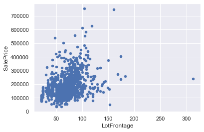
First, examine the plots of features versus target one by one and identify observations that do not follow the trend. Only these observations are outliers and not the ones following the trend but having a greater or smaller value.

首先，逐一检查特征与目标的关系图，并确定不遵循趋势的观察结果。只有这些观察值是异常值，而不是跟随趋势的值，具有较大或较小的值。

#Outliers in Fig 1 
df_train.sort_values(by = 'GrLivArea', ascending = False)[:2]
#Fig 2(Clockwise)
df_train.sort_values(by='TotalBsmtSF',ascending=False)[:2]
#fig 3 
df_train.drop(df_train[df_train['LotFrontage']>200].index,inplace=True)
#Fig 4
df_train.drop(df_train[(df_train.YearBuilt < 1900) & (df_train.SalePrice > 200000)].index,inplace=True)
# Fig 5
df_train.drop(df_train[(df_train.OverallQual==4) & (df_train.SalePrice>200000)].index

One might be tempted to delete the observations for LotArea above 100k. However, on second thought it is possible these were just large houses but overall low quality.

人们可能会想删除高于100k的LotArea的观测值。然而，再三考虑，这可能只是大房子，但总体质量低下。

df_train[df_train['LotArea']>100000]['OverallQual']Out []:
249    6
313    7
335    5
706    7

Thus, we see that despite having larger Lot Area, these houses have a overall quality of 7, and average price for that quality is a bit more than 200k as seen in the box plot. Thus, these houses may not be a harmful outlier to the model.

因此，我们看到，尽管地段面积较大，但这些房屋的整体质量为7，如箱形图中所示，该质量的平ASP格略高于200k。因此，这些房屋可能不会对模型造成有害影响。

Thus, we will see the correlations will have increased for the variables after removing outliers.

因此，我们将看到去除异常值后变量的相关性将增加。

2.特征工程 (2.Feature Engineering)

Concatenate the training and testing sets to create new features and fill in missing values so that number and scale of features remains same in both sets.

将训练和测试集连接起来以创建新特征并填写缺失值，以使两个集合中特征的数量和比例保持不变。

2.1。缺少数据 (2.1.Missing Data)

Thus, some features have too many missing values. These features can make our model over fit on the few values present.

因此，某些功能缺少太多的值。这些功能可以使我们的模型在现有的几个值上过拟合。

First, fill all the missing values for creating new features and later delete features where 97 % of the values are identical.

首先，填写所有缺少的值以创建新特征，然后删除其中97％的值相同的特征。

Some features are listed as numerical data whereas should be string data. These features are the Location features, MS Zoning,MSSubclass, YearBuilt, MoSold,etc. For other important features like LotFrontage, GarageArea, and MS Zoning fill in the median or mode values. As a last step, fill in all null values as None for string and 0 for numeric.

某些功能列为数字数据，而应为字符串数据。这些功能包括位置功能，MS分区，MSSubclass，YearBuilt，MoSold等。对于其他重要功能，例如LotFrontage，GarageArea和MS Zoning，请填写中位数或众数。最后一步，将所有空值填写为字符串(无)和数字(0)。

objects = []
for i in all_features.columns:
    if all_features[i].dtype == object:
        objects.append(i)
all_features.update(all_features[objects].fillna('None'))
numeric_dtypes = ['int16', 'int32', 'int64', 'float16', 'float32', 'float64']
numeric = []
for i in all_features.columns:
    if all_features[i].dtype in numeric_dtypes:
        numeric.append(i)
all_features.update(all_features[numeric].fillna(0))

2.2。新功能 (2.2.New features)

Creating features deemed to be relevant by subjective analysis of features, such as:

通过对功能进行主观分析来创建被认为相关的功能，例如：

1)Years since Remodelling of the house.

1)自房屋改建以来的年份。

2)Total surface area=Total basement surface area+ 1st Floor SF + 2nd Floor SF

2)总表面积=总地下室表面积+ 1楼SF + 2楼SF

3)Bathrooms =full bathrooms + 0.5* half bathrooms

3)浴室=完整浴室+ 0.5 *半浴室

4)Average Room Size= Ground living area / (Number of rooms and bathrooms)

4)平均房间大小=地面居住面积/(房间和浴室数量)

5)Bedroom Bathroom tradeoff = Bedrooms * Bathrooms

5)卧室浴室的权衡=卧室*浴室

6)Porch Area = Sum of porch features

6)门廊面积=门廊特征总和

7)Type of Porch = categorical feature

7)门廊类型=分类特征

8)The newness of the house captured by its age taking in factor of renovation.

8)房屋的新颖性受其年龄影响而受到翻修。

Some of the features were created in this way:

一些功能是通过这种方式创建的：

2.3。映射重要的分类特征 (2.3. Mapping important categorical features)

Basically, this is manually encoding the categorical features. Dummy variables or one hot encoding creates sparse matrices and does not capture the importance or relationship of the feature as we want it to. For example, the following map for neighborhoods feature encodes the categories according to their median sale price and we can encode more expensive areas as higher values to explore the relationship. Verify this by trying both methods, one hot encoding and the manual mapping, the latter scores significantly higher.

基本上，这是手动对分类特征进行编码。虚拟变量或一种热编码会创建稀疏矩阵，并且无法捕获我们想要的特征的重要性或关系。例如，下面的街区地图根据其中位数销售价格对类别进行编码，我们可以将价格较高的区域编码为较高的值来探索这种关系。通过尝试两种方法(一种是热编码和手动映射)来验证这一点，后者的得分要高得多。

# Mapping neighborhood unique values according to the shades of the box-plot
neigh_map={'None': 0,'MeadowV':1,'IDOTRR':1,'BrDale':1,
        'OldTown':2,'Edwards':2,'BrkSide':2,
        'Sawyer':3,'Blueste':3,'SWISU':3,'NAmes':3,
        'NPkVill':4,'Mitchel':4,'SawyerW':4,
        'Gilbert':5,'NWAmes':5,'Blmngtn':5,
        'CollgCr':6,'ClearCr':6,'Crawfor':6,
        'Somerst':8,'Veenker':8,'Timber':8,
         'StoneBr':10,'NoRidge':10,'NridgHt':10 } 
all_features['Neighborhood'] = all_features['Neighborhood'].map(neigh_map)
# Quality maps for external and basementbsm_map = {'None': 0, 'Po': 1, 'Fa': 4, 'TA': 9, 'Gd': 16, 'Ex': 25}
#ordinal_map = {'Ex': 10,'Gd': 8, 'TA': 6, 'Fa': 5, 'Po': 2, 'NA':0}
ord_col = ['ExterQual','ExterCond','BsmtQual', 'BsmtCond','HeatingQC',
           'KitchenQual','GarageQual','GarageCond', 'FireplaceQu']
for col in ord_col:
    all_features[col] = all_features[col].map(bsm_map)
all_features.shape

Impute negative values obtained from Years_Since_Remod in the test set as zero.

将从测试集中的Years_Since_Remod获得的负值估算为零。

all_features[all_features['YrSold'].astype(int) <      all_features['YearRemodAdd'].astype(int)]all_features.at[2284,'Years_Since_Remod']=0
all_features.at[2538,'Years_Since_Remod']=0
all_features.at[2538,'Age']=0

2.4。掉落功能 (2.4. Drop features)

2.5。功能缩放 (2.5. Feature Scaling)

Target Scaling

目标缩放

#The target is scaled to logarithmic distribution.
target = np.log1p(df_train['SalePrice']).reset_index(drop=True)

2.6特征变换，对数和二次关系 (2.6.Feature transformation, logarithmic and quadratic relationships)

Squaring and logging numeric features to explore degrees of relationships.

平方和记录数值特征以探索关系的程度。

Note: Use numeric list of training data set before encoding the categorical variables.

注意：在对分类变量进行编码之前，请使用训练数据集的数字列表。

Cubed and square root features were also used but did not result in significant improvement and led to over-fitting on including all features.

还使用了立方和平方根特征，但并未带来明显的改善，并导致对所有特征的过度拟合。

#Convert remaining categorical features by one hot encoding
all_features=pd.get_dummies(all_features).reset_index(drop=True)
all_features1=pd.get_dummies(all_features1).reset_index(drop=True)
loged_features=pd.get_dummies(loged_features).reset_index(drop=True)
log_sq_cols=pd.get_dummies(log_sq_cols).reset_index(drop=True)# Re-Split the training and testing data
def get_splits(all_features,target): 
    df=pd.concat([all_features,target],1)
    X_train=df.iloc[:len(target),:]
    X_test=all_features.iloc[len(target):,:]
    return X_train,X_test# Split for dataset containing log and squared features:
X_train1,X_test1=get_splits(log_sq_cols,target)
train1,valid1,feature_col1=get_valid(X_train1,'SalePrice')

2.7使用Lasso回归进行多变量分析 (2.7.Multi-variate analysis using Lasso Regression)

Lasso regression or the L1 penalty regularization is used for feature selection as undesired features are weighted zero as the alpha coefficient is increased.

套索回归或L1罚则正则化用于特征选择，因为不希望的特征随着alpha系数的增加而加权为零。

A wide range of alphas is used in cross validation and best model is selected. The corresponding weights of the features are extracted by using the .coef_ attribute of LassoCV.

交叉验证中使用了多种alpha，并选择了最佳模型。使用LassoCV的.coef_属性提取要素的相应权重。

3.岭回归 (3. Ridge Regression)

To predict the sales price of the training set houses, ridge regression is used on features obtained from Lasso model.

为了预测训练集房屋的销售价格，对从套索模型获得的特征使用了岭回归。

Ridge model using cross validation for the L2 alpha is performed using all the features in the log_sq_col list. One may perform ridge for all the lists obtained above and check that log_sq_col list obtains least CV score.

使用log_sq_col列表中的所有功能执行针对L2 alpha使用交叉验证的Ridge模型。一个人可以对上面获得的所有列表执行岭，并检查log_sq_col列表获得的CV得分最低。

Ridge regression using cross validation is performed for various number of features using the sorted list from Lasso model. It is observed that the model generalizes best when 270 features are included. A more extensive search over number of features can be performed but result is same.

使用来自Lasso模型的排序列表，对各种数量的要素执行使用交叉验证的Ridge回归。可以看出，当包含270个特征时，该模型的泛化效果最佳。可以对特征数量进行更广泛的搜索，但结果相同。

4.推论 (4. Inferences)

The ridge regression model with 270 features and alpha of 21 is the best regression model for given training set and gives the lowest test set error. Thus in this section we will try to find which features are generally important for predicting sale price and which the model has chosen and resulted in improved score.

对于给定的训练集，具有270个特征且alpha为21的岭回归模型是最佳回归模型，并且给出了最低的测试集误差。因此，在本节中，我们将尝试找出通常对于预测销售价格而言重要的特征，以及选择了哪些模型并提高得分的模型。

Feature importance is calculated using Permutation importance from eli5 library. This function calculates the change in the target variable while keeping other features constant.

使用eli5库中的置换重要性来计算特征重要性。该函数在保持其他功能不变的情况下计算目标变量的变化。

First the importance given by using the default features provided in the train set,

首先，通过使用火车集中提供的默认功能来赋予重要性，

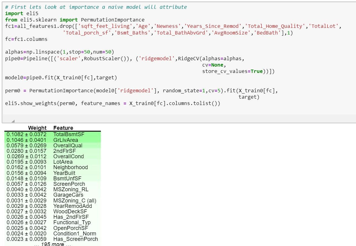
Thus we see a naive model using all the features provided gives importance to space features like Basement, Grade living area and 2nd Floor surface area. Also, neighborhood and year built features are also present.

因此，我们看到使用所有提供的功能的幼稚模型都对诸如地下室，坡度居住区域和2楼表面积等空间特征非常重要。此外，还提供邻里和年份构建功能。

The importance imputed by the ridge model formed above with 270 features,

由上面形成的具有270个要素的山脊模型推定的重要性，

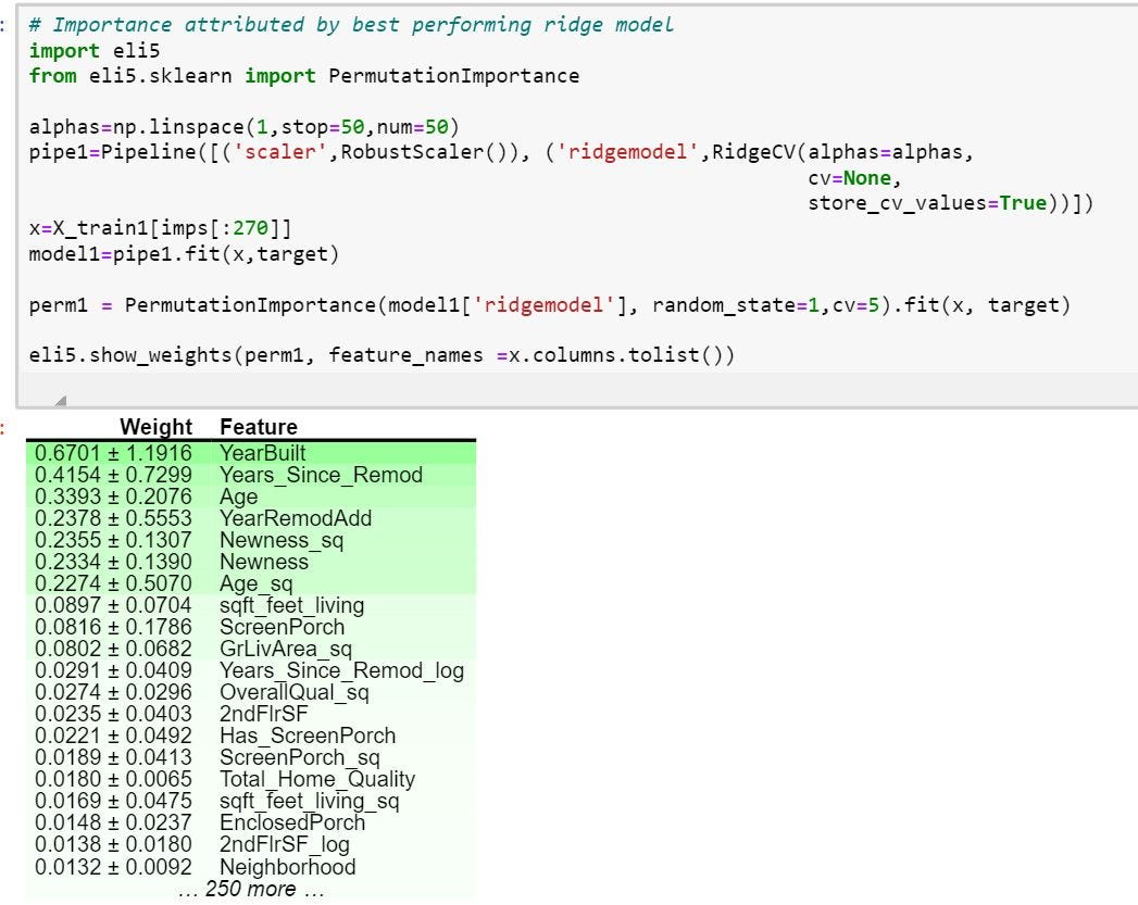
Thus, one can observe that the ridge model gives the time related features more weight than space features. One reason can be that in the naive model, there were not enough time features as much as space features, and time features are of lower absolute value having lower impact.

因此，可以观察到，与空间特征相比，山脊模型赋予与时间相关的特征更大的权重。一个原因可能是在天真的模型中，没有足够的时间特征和空间特征，并且时间特征的绝对值较低，影响较小。

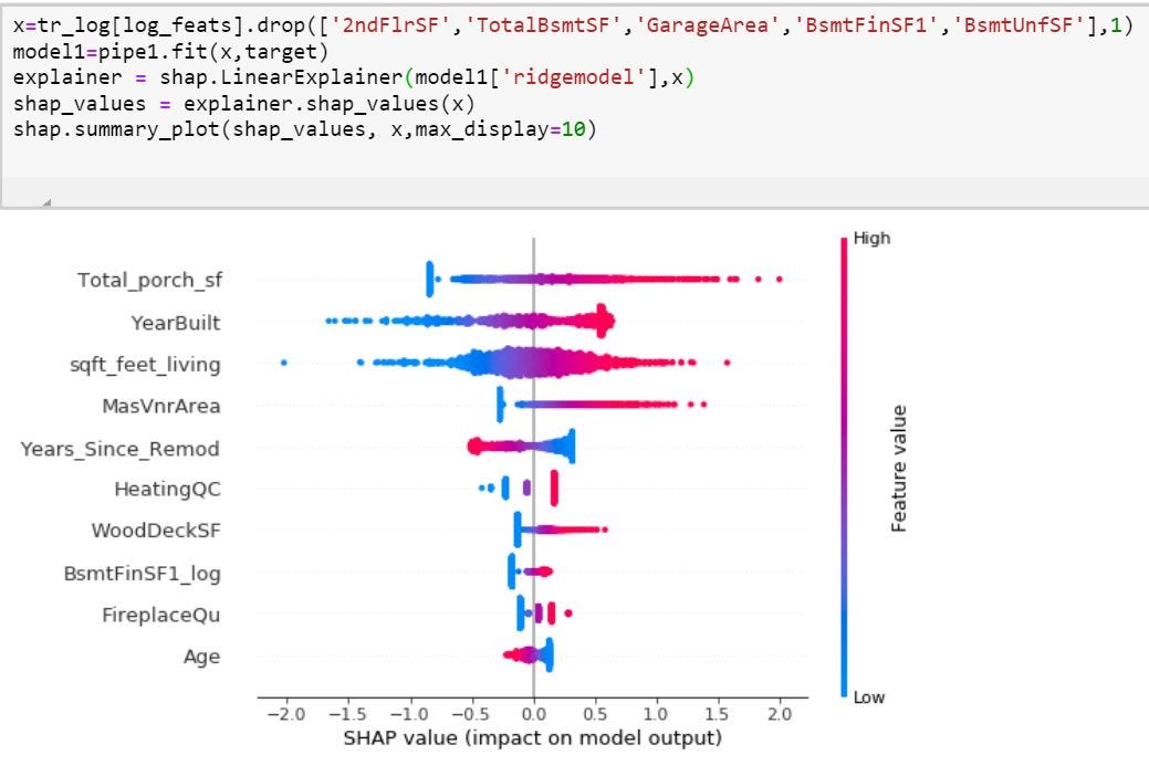
To observe impact of the change in features on the target, we plot the summary plot of the shap values.

为了观察特征变化对目标的影响，我们绘制了shap值的摘要图。

Naturally the sale price is impacted greatly by house having a large 2nd floor area which also indicates the house has large ground floor area. Moreover, it is a numeric squared feature having high absolute values.

自然，销售价格受第二层面积较大的房屋的影响很大，这也表明该房屋的第二层面积较大。而且，它是具有高绝对值的数字平方特征。

To observe impact on output of other features, we can drop the space features or only use the particular features intended.

要观察对其他要素输出的影响，我们可以删除空间要素或仅使用预期的特定要素。

5，结论 (5.Conclusion)

That’s the end of the exercise. The prices have been predicted upto a tolerance of 12,000 dollars for a median price of 162,000. The important features have been explored and insights can be drawn to modify and sell houses at a higher price.

练习到此结束。预计价格最高可容忍12,000美元，中位数价格为162,000。已经探索了重要的功能，并且可以得出见识以修改和以更高的价格出售房屋。

Certainly one can use other models to obtain the shap values and explore the feature importance. However, you will need tensorflow package or 3.8 version of Python to perform that. Besides, other models do not perform as well as Ridge, only used to increase the submission score by blending.

当然，可以使用其他模型来获取形状值并探索特征的重要性。但是，您将需要tensorflow软件包或3.8版本的Python来执行此操作。此外，其他模型的效果不及Ridge，仅用于通过混合来提高提交分数。

Note: It is not recommended to use data leakage for gaining real practical experience and many notebooks found on the competition dashboard use it in between the modelling cells without mentioning. Thus, it should be noted this notebook does not use data leakage and neither do any of the given references.

注意：建议不要使用数据泄漏来获得实际的实践经验，并且比赛仪表板上的许多笔记本都在建模单元之间使用数据泄漏而没有提及。因此，应该注意的是，该笔记本电脑不使用数据泄漏，也没有使用任何给定的参考文献。

References for the notebook:

笔记本参考：

For understanding of features and introduction:

为了了解功能和介绍：