多边形网格数据结构_网格数据结构

最新推荐文章于 2024-07-13 12:01:32 发布

weixin_26750481

最新推荐文章于 2024-07-13 12:01:32 发布

阅读量1.5k

点赞数 1

文章标签：数据结构 python java

原文链接：https://towardsdatascience.com/mesh-data-structure-d8b1a61d749e

版权

本文介绍了多边形网格数据结构，它是计算机图形学中用于表示三维形状的重要工具。通过翻译自的数据科学文章深入探讨了其概念和应用。

摘要由CSDN通过智能技术生成

多边形网格数据结构

For surface networks, the important feature is the topology, rather than the location of its vertices. Different topologies have created different data structures and standards. Different topologies have different performances for grid query and editing.

对于地面网络，重要的功能是拓扑，而不是其顶点的位置。不同的拓扑创建了不同的数据结构和标准。不同的拓扑对于网格查询和编辑具有不同的性能。

For digital media, games, real-time interaction, etc., models are usually irregular curved geometry, which requires aesthetics and short enough calculation time. Therefore, the model is usually a discretized surface mesh. The so-called discretization is a mesh that is spliced by a series of patches, which seems to be rough, but it can be made smooth through texture and rendering technology.

对于数字媒体，游戏，实时交互等，模型通常是不规则的弯曲几何形状，这需要美观并且需要足够短的计算时间。因此，模型通常是离散的表面网格。所谓离散化是一种由一系列补丁拼接而成的网格，看似粗糙，但可以通过纹理和渲染技术使其变得平滑。

The half-edge data structure is a slightly complicated edge representation method and all proximity queries can be done in constant time. Even better if the adjacency information of faces, vertices and edges is included, the size of the data structure is fixed and compact.

半边数据结构是一种稍微复杂的边表示方法，所有邻近查询都可以在恒定时间内完成。如果包括面，顶点和边的邻接信息，则更好，数据结构的大小是固定且紧凑的。

The basic elements of the half-edge data structure are vertices, faces and half-edges.

半边数据结构的基本元素是顶点，面和半边。

Each edge is divided into two halves, and each half-edge is a directed edge with opposite directions. If an edge is shared by two faces, each face can have a half. It can be seen that for a half-edge mesh, three structures need to be implemented:

每个边缘均分为两半，每个半边缘是方向相反的有向边缘。如果一条边由两个面共享，则每个面可以有一半。可以看出，对于半边网格，需要实现三个结构：

Vertex that stores the (x, y, z) coordinates.
存储(x，y，z)坐标的顶点。
Face that contains all the indexes of the vertices that make up the face.
包含组成面的所有顶点索引的面。
Half-edge that Contains the index of the end point , the adjacent face , the next half edge , and the opposite edge
包含端点，相邻面，下一个半边和相对边的索引的半边

class HalfEdge( object ):
   def __init__( self ):
     self.to_vertex = -1
     self.face = -1
     self.edge = -1
     self.opposite_he = -1
     self.next_he = -1

The implementation here simplifies some content, such as the texture coordinates of the vertices, normals, etc.

这里的实现简化了一些内容，例如顶点的纹理坐标，法线等。

Most answers to proximity queries are stored in data structures of edges, points, and faces. For example, the faces or points surrounding the half can be easily found.

邻近查询的大多数答案都存储在边，点和面的数据结构中。例如，可以轻松找到围绕一半的面或点。

def vertex_face_neighbors( self, vertex_index ):
   halfedges = self.halfedges
   result = []
   start_he = halfedges[ self.vertex_halfedges[ vertex_index ] ]
   he = start_he
   while True:
      if -1 != he.face: 
         result.append( he.face )
         he = halfedges[ halfedges[ he.opposite_he ].next_he ]
         if he is start_he: 
            break
    return resultdef vertex_vertex_neighbors( self, vertex_index ):    halfedges = self.halfedges
    result = []
    start_he = halfedges[ self.vertex_halfedges[ vertex_index ] ] 
    he = start_he
    while True:
       result.append( he.to_vertex )
       he = halfedges[ halfedges[ he.opposite_he ].next_he ]
       if he is start_he:
           break
    return result

To be able to calculate the neighboring faces the neighboring vertices needs to be found first.

为了能够计算相邻面，首先需要找到相邻顶点。

We start from the current vertex (V_0), we step ahead with the halfedge next pointer to the ring surrounding the current vertex.

我们从当前顶点(V_0)开始，然后向前移动半边沿的下一个指针，指向当前顶点周围的环。

Once out in the ring the only thing that needs to be done is to store the vertex index and step ahead with the half-edge next pointer until it points to the starting vertex in the ring.

一旦进入环中，唯一要做的就是存储顶点索引并向前移动半边的下一个指针，直到它指向环中的起始顶点为止。

The neighboring faces is done by using this ring of surrounding vertices and check their corresponding faces. Because every half-edge stores the left face it is easily retrieved by looping through the neighboring vertices and putting all neigboring faces indices into a vector.

相邻的面是通过使用此环的周围顶点完成的，并检查它们对应的面。由于每个半边都存储左脸，因此可以通过遍历相邻顶点并将所有相邻的脸索引放入向量中来轻松检索。

We can implements a simple Half-Edge based on a triangular mesh from OBJ file Format OFF that contains :

我们可以基于OBJ文件Format OFF中的三角形网格实现一个简单的Half-Edge，该三角形网格包含：

Number of vertices s
顶点数s
Number of faces c
面数c
Description of the faces (sequence of the indices of the vertices of the face, preceded by its number of vertices).
面的描述(面顶点索引的顺序，其顶点数量开头)。

First we read all the vertex coordinate information,then we read the surface information to create the surface.

首先，我们读取所有顶点坐标信息，然后读取表面信息以创建表面。

def TriMesh_FromOBJ( path ):
   result = TriMesh()
   obj_lines = open( path )
   n_v,n_f,_=[int(u) for u in next(obj_lines).split()]
   for i in range(n_v):
      result.vs.append([float(u) for u in next(obj_lines).split()])
   for i in range(n_f):
      result.faces.append([float(u) for u in next(obj_lines).split()[1:]])   obj_lines.close()
   result.vs=np.array(result.vs)
   result.faces=np.array(result.faces,dtype=int)
   return result

Perhaps the biggest difficulty encountered in realizing half-edge structure is how to efficiently realize the link relationship between an edge and its dual edge.

实现半边结构时可能遇到的最大困难是如何有效地实现边和其双边之间的链接关系。

First we create all the faces, regardless of the problem of dual sides, we wait until all the faces and halves are created, and then perform a unified operation on all the edges to find the dual side of each half.

首先，我们创建所有面，而不考虑双面的问题，我们等到创建所有面和两半后，再对所有边执行统一操作，以找到每半边的双面。

def update_halfedges( self ):   self.halfedges = []
   self.vertex_halfedges = None
   self.face_halfedges = None
   self.edge_halfedges = None
   self.directed_edge2he_index = {}
   __directed_edge2face_index = {}
   for fi, face in enumerate( self.faces ):
      __directed_edge2face_index[ (face[0], face[1]) ] = fi   
      __directed_edge2face_index[ (face[1], face[2]) ] = fi
      __directed_edge2face_index[ (face[2], face[0]) ] = fi   def directed_edge2face_index( edge ):
      result = __directed_edge2face_index.get( edge, -1 )
      if -1 == result:
           assert edge[::-1] in __directed_edge2face_index
      return result   self.vertex_halfedges = [None] * len( self.vs )  
   self.face_halfedges = [None] * len( self.faces )     self.edge_halfedges = [None] * len( self.edges )   for ei, edge in enumerate( self.edges ):      he0 = self.HalfEdge()
      he0.face = directed_edge2face_index( edge )
      he0.to_vertex = edge[1]
      he0.edge = ei
      he1 = self.HalfEdge()
      ## The face will be -1 if it is a boundary half-edge.
      he1.face = directed_edge2face_index( edge[::-1] )
      he1.to_vertex = edge[0]
      he1.edge = ei
      he0index = len( self.halfedges )
      self.halfedges.append( he0 )
      he1index = len( self.halfedges )
      self.halfedges.append( he1 )      he0.opposite_he = he1index
      he1.opposite_he = he0index
      self.directed_edge2he_index[ edge ] = he0index      self.directed_edge2he_index[ edge[::-1] ] = he1index

The face has 3 halves. When creating these 3 halves every time, the dual edges are also created in advance, and the dual relationship is directly linked.

脸部分为三半。每次创建这三个半部分时，也会预先创建双重边缘，并且双重关系直接关联。

The face is then created and the half-edge pair and normal is connected to the face. The normal is calculated as follows ,

然后创建面并将半边对和法线连接到该面。正常值计算如下：

Where v1, v2 and v3 are the vertices spanning up the face,

其中v1，v2和v3是横跨整个面的顶点，

And then it is then normalized.

然后将其标准化。

def update_face_normals_and_areas( self ):
    self.face_normals = np.zeros( ( len( self.faces ), 3        self.face_areas = np.zeros( len( self.faces ) )
    vs = np.asarray( self.vs )
    fs = np.asarray( self.faces, dtype = int )
    self.face_normals = np.cross( vs[ fs[:,1] ] - vs[ fs[:,0] ], vs[   fs[:,2] ] - vs[ fs[:,1] ] ) 
    self.face_areas = np.sqrt((self.face_normals**2).sum(axis=1))
    self.face_normals /= self.face_areas[:,np.newaxis]     self.face_areas *= 0.5

The area of the i-th face is calculated as half the magnitude of the cross product between the edges in the i-th face.

第i个面的面积计算为第i个面的边缘之间的叉积的一半。

The vertex normal is also calculated as follows,

顶点法线也如下计算：

Which is the normalized sum of the neighboring face normals,

这是相邻人脸法线的标准化总和，

def update_vertex_normals( self ):
   self.vertex_normals = np.zeros( ( len(self.vs), 3 ) )
   for vi in range( len( self.vs ) ):.
      for fi in self.vertex_face_neighbors( vi ):         self.vertex_normals[vi] += self.face_normals[ fi ] *      
self.face_areas[ fi ]
    self.vertex_normals *= 1./np.sqrt( ( self.vertex_normals**2 ).sum(1) ).reshape( (len(self.vs), 1) )

After creating the Half-edge structure, we can use the OpenGl library to render the mesh 3D.

创建Half-edge结构后，我们可以使用OpenGl库渲染3D网格。

import pygame
from pygame.locals import *
from OpenGL.GL import *
from OpenGL.GLU import *result=TriMesh_FromOBJ( "cube.off")
result.update_edge_list( )
result.update_halfedges()verticies=result.vs
edges=result.edgesdef Mesh():
  glBegin(GL_LINES)
  for edge in edges:
   for vertex in edge:
    glVertex3fv(verticies[vertex])
  glEnd()def main():
  pygame.init()
  display = (800,600)
  pygame.display.set_mode(display, DOUBLEBUF|OPENGL)
  gluPerspective(45, (display[0]/display[1]), 0.1, 50.0)
  glTranslatef(0.0,0.0, -5)
  while True:
    for event in pygame.event.get():
      if event.type == pygame.QUIT:
          pygame.quit()
          quit()
    glRotatef(1, 3, 1, 1)
    glClear(GL_COLOR_BUFFER_BIT|GL_DEPTH_BUFFER_BIT)
    Mesh()
    pygame.display.flip()
    pygame.time.wait(10)

The simplest mesh example is the 3D cube,

最简单的网格示例是3D立方体，

Where the green line represent the normal surface and the red line represent the vertex normal.

绿线代表法线表面，红线代表顶点法线。

离散微分算子 (Discrete Differential Operators)

Let S be a surface embedded in R³ , described by an arbitrary parameterization of 2 variables.

设S为嵌入R 3中的表面，用2个变量的任意参数化描述。

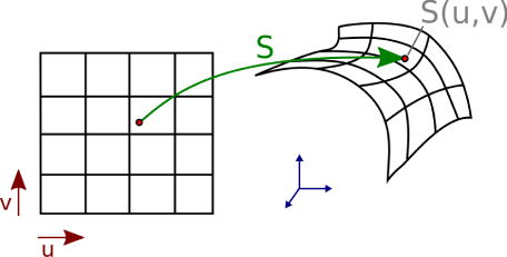
For each point on the surface S, we can locally approximate the surface by its tangent plane, orthogonal to the normal vector n. Local bending of the surface is measured by curvatures. For every unit direction in the tangent plane, the normal curvature κ^N (θ) is defined as the curvature of the curve that belongs to both the surface itself and the plane containing both n and the tangent vectors .

对于表面S上的每个点，我们可以通过与法线向量n正交的切线平面局部近似表面。表面的局部弯曲通过曲率来测量。对于切平面中的每个单位方向，法线曲率κ^ N(θ)定义为曲线的曲率，该曲率既属于曲面本身，又属于包含n和切线向量的平面。

The two principal curvatures κ_1 and κ_2 of the surface S, with their associated orthogonal directions are the extremum values of all the normal curvatures.

曲面S的两个主曲率κ_1和κ_2及其相关的正交方向是所有法线曲率的极值。

The mean curvature κ_H is defined as the average of the normal curvatures:

平均曲率κ_H定义为法向曲率的平均值：

Expressing the normal curvature in terms of the principal curvatures,

用主曲率表示法向曲率，

Leads to the well-known definition:

导致众所周知的定义：

Since the triangle mesh is meant to visually represent the surface, we select a linear finite element on each triangle, a linear interpolation between the three vertices corresponding to each triangle. Then, for each vertex, an associated surface patch , over which the average will be computed, we will denote the surface area as A_M.

由于三角形网格的目的是可视化地表示表面，因此我们在每个三角形上选择一个线性有限元，即在对应于每个三角形的三个顶点之间进行线性插值。然后，对于每个顶点，一个相关的表面斑块(将在其上计算平均值)将表面积表示为A_M。

Since the mean curvature normal operator is a generalization of the Laplacian from flat spaces to manifolds, we first compute the Laplacian of the surface with respect to the conformal space parameters u and v, we use the current surface discretization as the conformal parameter space, for each triangle of the mesh, the triangle itself defines the local surface metric.

由于平均曲率法线算子是从平面空间到流形的拉普拉斯算子的推广，因此我们首先针对保形空间参数u和v计算表面的拉普拉斯算子，我们将当前表面离散化用作保形参数空间，对于网格的每个三角形，三角形本身都定义了局部表面度量。

With such an induced metric, the operator simply turns into a Laplacian

通过这种归纳度量，操作员可以简单地转换为拉普拉斯算子

Using Gauss’s theorem, the integral over a surface going through the midpoint of each 1-ring edge of a triangulated domain can be expressed as a function of the node values and the angles of the triangulation.

使用高斯定理，经过三角区域的每个1环边缘的中点的表面上的积分可以表示为节点值和三角角度的函数。

The integral thus reduces to the following simple form:

积分因此简化为以下简单形式：

where α and β are the two angles opposite to the edge in the two triangles sharing the edge (x_i, x_j ),

其中α和β是在共享边(x_i，x_j)的两个三角形中与边相对的两个角度，

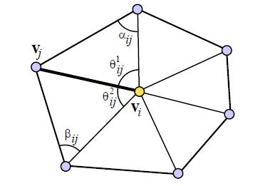
And N_1(i) is the set of 1-ring neighbor vertices of vertex i.

N_1(i)是顶点i的1环相邻顶点的集合。

We can express the mean curvature normal operator K defined in Section 2.1 using the following expression:

我们可以使用以下表达式表示第2.1节中定义的平均曲率法线算子K：

Where A is the non-obtuse Voronoi area for a vertex x_i as a function of the neighbors x_j defined as follows :

其中A是顶点x_i的非钝Voronoi区域，它是邻居x_j的函数，定义如下：

If your mesh is represented with an half-edge data structure the pseudo code to compute K is:

如果您的网格用半边数据结构表示，则用于计算K的伪代码为：

numv = vertices.shape[0]
numt = triangles.shape[0]self.A = np.zeros((numv, numt))
self.L = np.zeros((numv, numt, 3))for i in range(numv):
   req_t = triangles[(triangles[:, 0] == i) | (triangles[:, 1] == i)   | (triangles[:, 2] == i)]
   for j in range(len(req_t)):
        tid = np.where(np.all(triangles == req_t[j], axis=1))
        nbhr = [v for v in req_t[j] if v != i]
        vec1 = (vertices[nbhr[0]] - vertices[i]) /   np.linalg.norm(vertices[nbhr[0]] - vertices[i], 2) 
        vec2 = (vertices[nbhr[1]] - vertices[i]) /                np.linalg.norm(vertices[nbhr[1]] - vertices[i], 2)       angle_at_x = np.arccos(np.dot(vec1, vec2))
       if angle_at_x > np.pi / 2:
           self.A[i, tid] = get_heron_area(vertices[i], vertices[nbhr[0]], vertices[nbhr[1]]) / 2           continue       vec1a = (vertices[i] - vertices[nbhr[0]]) / np.linalg.norm(vertices[i] - vertices[nbhr[0]], 2)       vec2a = (vertices[nbhr[1]] - vertices[nbhr[0]]) /    np.linalg.norm(vertices[nbhr[1]] - vertices[nbhr[0]], 2)       inner_prod = np.dot(vec1a, vec2a)
       angle1 = np.arccos(inner_prod)
       if angle1 > np.pi / 2:
          self.A[i, tid] = get_heron_area(vertices[i], vertices[nbhr[0]], vertices[nbhr[1]]) / 4          continue
       vec1b = (vertices[i] - vertices[nbhr[1]]) / \
np.linalg.norm(vertices[i] - vertices[nbhr[1]], 2)       vec2b = (vertices[nbhr[0]] - vertices[nbhr[1]]) / np.linalg.norm(vertices[nbhr[0]] - vertices[nbhr[1]], 2)      inner_prod = np.dot(vec1b, vec2b)
      angle2 = np.arccos(inner_prod)
      if angle2 > np.pi / 2:
         self.A[i, tid] = get_heron_area(vertices[i], vertices[nbhr[0]], vertices[nbhr[1]]) / 4         continue
      cot_1 = 1 / np.tan(angle1)
      cot_2 = 1 / np.tan(angle2)
      A_v_of_tid = 0.125 * ((cot_1 * np.linalg.norm(vertices[i] - vertices[nbhr[1]], 2)**2) + (cot_2 * np.linalg.norm(vertices[i] - vertices[nbhr[0]], 2)**2))      self.L_at_v_t = ((1 / np.tan(angle1)) * (vertices[i] - vertices[nbhr[1]])) + ((1 / np.tan(angle2)) * (vertices[i] - vertices[nbhr[0]]))       self.A[i, tid] = A_v_of_tid
       self.L[i, tid] = self.L_at_v_t
self.A = np.sum(self.A, axis=1)
# Set zeros in self.A to very small values
self.A[self.A == 0] = 10 ** -40
self.L = ((1 / (2 * self.A)) * np.sum(self.L, axis=1).T).T
self. K_H = 0.5 * np.linalg.norm(self.L, 2, axis=1)

Curvature is a quantity describing the degree of curvature of a geometric body, such as the degree of deviation of a three-dimensional curved surface from a plane, or the degree of deviation of a two-dimensional curve from a straight line, and can also determine the type of curved surface. Often used in geometric analysis, geographic surveying and mapping and other fields.

曲率是描述几何体的曲率程度的量，例如三维曲面相对于平面的偏离程度或二维曲线相对于直线的偏离程度，并且也可以确定曲面的类型。常用于几何分析，地理测绘等领域。

The arithmetic average of the two principal curvatures describes the curvature of an embedded surface in some ambient space such as Euclidean space. The mean curvature is positive and locally concave. The mean curvature is negative and locally convex.

两个主曲率的算术平均值描述了某些环境空间(例如欧几里得空间)中嵌入表面的曲率。平均曲率是正的并且局部凹入。平均曲率是负的并且局部凸。

Mark Meyer, Mathieu Desbrun, Peter Schr¨oder, and Alan H. Barr.Discrete Differential-Geometry Operators for Triangulated 2-Manifolds.
马克·迈耶(Mark Meyer)，马修·德斯布伦(Mathieu Desbrun)，彼得·施罗德(Peter Schroder)和艾伦·巴尔(Alan H.Barr)。三角二维流形的离散差分几何算子
Keenan Crane.DISCRETE DIFFERENTIAL GEOMETRY: AN APPLIED INTRODUCTION
Keenan Crane。离散微分几何：应用导论
Do Carmo, Manfredo (2016). Differential Geometry of Curves and Surfaces (Second ed.). Dover. p. 158. ISBN 978–0–486–80699–0.
曼弗雷多·卡莫(2016)。 曲线和曲面的微分几何 (第二版)。多佛 p。 158. ISBN 978–0–486–80699-0 。
Goldman, R. (2005). “Curvature formulas for implicit curves and surfaces”. Computer Aided Geometric Design. 22 (7): 632–658. doi:10.1016/j.cagd.2005.06.005.
Goldman，R.(2005年)。 “隐式曲线和曲面的曲率公式”。 计算机辅助几何设计 。 22 (7)：632-658。 doi ： 10.1016 / j.cagd.2005.06.005 。
Spivak, M (1975). A Comprehensive Introduction to Differential Geometry. 3. Publish or Perish, Boston.
Spivak，M(1975)。 微分几何概论 。 3 。出版或灭亡，波士顿。
Rosenberg, Harold (2002), “Bryant surfaces”, The global theory of minimal surfaces in flat spaces (Martina Franca, 1999), Lecture Notes in Math., 1775, Berlin: Springer, pp. 67–111, doi:10.1007/978–3–540–45609–4_3, ISBN 978–3–540–43120–6, MR 1901614.
罗森伯格 ( Rosenberg)，哈罗德 ( Harold) (2002)，“布赖恩特曲面”， 平坦空间中最小曲面的全局理论(马丁纳·弗兰卡，1999年) ，数学讲义， 1775年 ，柏林：施普林格，第67–111页， doi ： 10.1007 / 978–3–540–45609–4_3 ， ISBN 978–3–540–43120–6 ， MR 1901614 。
The definition of a DCEL may be found in all major books in computational geometry.
DCEL的定义可以在计算几何学的所有主要书籍中找到。
Muller, D. E.; Preparata, F. P. “Finding the Intersection of Two Convex Polyhedra”, Technical Report UIUC, 1977, 38pp, also Theoretical Computer Science, Vol. 7, 1978, 217–236
德州穆勒； FP，Preparata，“发现两个凸多面体的交点”， UIUC技术报告，1977年，38pp， 理论计算机科学 ，第1卷。 7，1978，217–236
de Berg, Mark (1997). Computational Geometry, Algorithms and Applications, Third Edition. Springer-Verlag Berlin Heidelberg. p. 33. ISBN 978–3–540–77973–5.
马克·德·伯格(1997)。 计算几何，算法和应用，第三版 。施普林格出版社柏林海德堡。 p。 33. ISBN 978–3–540–77973–5 。