SVD vs PCA vs 1bitMC

EigenDecomposition

For any real symmetric square $d\times d$ matrix A , we can find its eigenvalues ${\lambda }_1\ge {\lambda }_2\ge ...\ge {\lambda }_d$ and corresponding orthonormal eigenvectors, such that:

$A{x}_1={\lambda }_1{x}_1$

$A{x}_2={\lambda }_1{x}_2$
…
$A{x}_d={\lambda }_1{x}_d$

• Suppose there are only m different non-zero eigenvalues, so we have

$A{x}_1={\lambda }_1{x}_1$

$A{x}_2={\lambda }_1{x}_2$
…
$A{x}_r={\lambda }_1{x}_r$

which can be written into a compact form such as ($U^T=U^{-1}$ and ($U{U}^T=I$):

$$A=U\Sigma U^T\text{\hspace{1em}(1)}$$

$$\Sigma =UA{U}^T\text{\hspace{1em}(2)}$$
Then we use above matrix $A$ to tranform a vector x, then

$$\begin{array}{rl}Ax& =U\Sigma U^{T}x\\ & =\left[\begin{array}{ccc}{x}_1& x_2\cdots & x_r\end{array}\right]\left[\begin{array}{ccc}{\lambda }_1& & \\ & \ddots & \\ & & {\lambda }_r\end{array}\right]\left[\begin{array}{c}{x}_1^T\\ x_2^T\\ \cdots \\ x_r^T\end{array}\right]x\end{array}$$

Start the calculation from right to left:

1. Re-Orient: Apply $U^T$ on x <==> dot proct of x with each rows of $U^T$. x will be projected on each orthonormal basis (new coordinate) which are the rows of the $U^T$. The geometric meaning of $U^{T}x$ is equivalent to rotate x based on the new cordinate (orthonormal basis) in $U^T$ .
2. $\Sigma U^{T}x$ is to use $\Sigma$ to extend or shrink the rotated $x$ along with the new coordinate. (If there is one $\lambda$=0, then that dimension will be removed. )
3. Re-Orient(to original):Same meaning with $U^T$. $U$ will rotate back x to original coordinate.
   

PCA

Main idea: Find a coordinate transformation matrix P applied on data suc that
(一种直观的看法是：希望投影后的投影值尽可能分散。数据越分散，可分性就越强，可分性越强，概率分布保存的就越完整)

1. The variability of the transformed data can be explained as much as possible along the new coordinates (降维后的信息损失尽可能小，尽可能保留原始样本的概率分布)

2. For each new coordinate, they should be orthoganal to each other to avoid the redundancy. (降维后的基之间是完全正交的)

3. So the final objective function is:
   $$\underset{P\in R^{m,d},U\in R^{d,m}}{\mathrm{argmin}}\sum _{i=1}^n||x_i-UP{x}_i|{|}_2^2\text{\hspace{1em}(*)}$$
   , where d is the original dimension of data and m is the new dimension of the transoformed data (r=rank(A) <=m ), $x_1,...,x_n\in R^d$ , $P\in R^{d,m}$ is the transformation of new coordinate, $U\in R^{d,m}$ (in the end $U=P^T$)is the transoformation of original coordinate.

4. In order to figure out above problems, the essential idea is to maxmize the variances of transfomred data point projected on new coordinates, and at the same time we need to minimize the covariance between two different coordinates(orthogonal<==>covarince is 0). Therefore, equivalently, we can diagolize the symmetric covariance matrix of the transformed data.

• Example (Let d =2).

Put data into matrix X:

$X=\left[\begin{array}{c}{x}_1,x_2,...,x_n\end{array}\right]=\left[\begin{array}{cccc}{a}_1& a_2& ...& a_n\\ b_1& b_2& ...& b_n\end{array}\right]\in R^{d=2,n}$

Suppose the data points has been centralized among each features. Therefore, the covariance matrix is the following:

$A=\frac{1}{n}X{X}^T=\left[\begin{array}{cc}\frac{1}{n}{\sum }_{i=1}^n{a}_i^2& \frac{1}{n}{\sum }_{i=1}^n{a}_i{b}_i\\ \frac{1}{n}{\sum }_{i=1}^n{a}_i{b}_i& \frac{1}{n}{\sum }_{i=1}^n{b}_i^2\end{array}\right]$

Transformed data by matrix P is $Y=PX$, where $P\in R^{m,d=2}$. Then the transofrmed covariance matrix is:

$$\begin{array}{rl}\frac{1}{n}Y{Y}^T& =\frac{1}{n}(PX)(PX{)}^T\\ & =\frac{1}{n}PX{X}^T{P}^T\\ & =P(\frac{1}{n}X{X}^T)P^T\\ & =PA{P}^T\end{array}$$

Once the minimization (*) is done , $\frac{1}{n}Y{Y}^T$ will look like $\Sigma$. Underline technique used to achieve the goal is the formula (2) , so that
$$\begin{array}{rl}PA{P}^T& =\Sigma \\ & =\left[\begin{array}{ccc}{\lambda }_1& & \\ & \ddots & \\ & & {\lambda }_m\end{array}\right]\end{array}$$

equivalently, $$A=P^T\Sigma P$$

where ${\lambda }_1={\sigma }_1^2\ge {\lambda }_2={\sigma }_2^2\ge ...\ge {\lambda }_m={\sigma }_m^2$, their corresponding eigenvectors construct the transformation matrix $P=\left[\begin{array}{c}{u}_1^T\\ u_2^T\\ ...\\ u_m^T\end{array}\right]\in R^{m,d=2}$, depends on your problems, we can select different r<=m rows in P.

SVD

$A$ will not be a symmetric matrix but with $m\times n$ dimension.
注意(SVD)： Original Feature is n (the number of colmns), New Feature is m
注意(PCA above) ： Original Feature is m (the number of rows)

Formula of Singular Value Decomposition
$$A_{m,n}=U\Sigma V^T$$

The main word of SVD is trying to solve the following two tasks:

1. First, find a set of orthonormal bais in n dimensional space
2. Second, once performed on above space, the resulting basis in m dimensional space are still orthonormal.

Suppose we have already got the set of orthonormal bais in n dimensional space $$V_{n,n}=\left[v_1,v_2,...,v_n\right]$$ (note: some vs can be 0 vectors), where $$v_i\perp v_j$$

Project A on n dimensional bais, we have:
$$\left[A{v}_1,A{v}_2,...,A{v}_n\right]$$

1. To make the projected basis be orthogonal as well, we need let the following happen:
   $$\begin{array}{rl}A{v}_i\cdot A{v}_j& =(A{v}_i{)}^{T}A{v}_j\\ & =v_i^T{A}^{T}A{v}_j\\ & =0\end{array}$$
   Therefore, if $v_{i}s$ are eigen vectors of $A^{T}A$, then the resulting projected basis are also orthogonal because:
   $$\begin{array}{rl}A{v}_i\cdot A{v}_j& =(A{v}_i{)}^{T}A{v}_j\\ & =v_i^T(A^{T}A{v}_j)\\ & =v_i^T{\lambda }_j{v}_j\\ & =0\end{array}$$

2. To scale the projected orthogonal basis into unit length.
   We have
   $$\begin{array}{rl}{u}_i& =\frac{A{v}_i}{|A{v}_i|}\\ & =\frac{A{v}_i}{\sqrt{|A{v}_i{|}^2}}\\ & =\frac{A{v}_i}{\sqrt{(A{v}_i{)}^{T}A{v}_i)}}\\ & =\frac{A{v}_i}{\sqrt{v_i^T(A^{T}A{v}_i)}}\\ & =\frac{A{v}_i}{\sqrt{v_i^T{\lambda }_i{v}_i}}(note:v_i^T{v}_i=1)\\ & =\frac{A{v}_i}{\sqrt{{\lambda }_i}}\end{array}$$

$$u_i\sqrt{{\lambda }_i}=u_i{\sigma }_i=A{v}_i,$$, where ${\sigma }_i=\sqrt{{\lambda }_i}$ is called singular value, $0\le i\le r$, r=rank(A).

3. In the end, we expand $\left[u_1,u_2,...,u_r\right]$ to $\left[u_1,u_2,...,u_r|u_{r+1},...,u_m\right]$ and select $\left[v_{r+1},v_{r+1},...,v_m\right]$ from the nullspace of A where $A{v}_i=0$, i>r, and ${\sigma }_i=0$
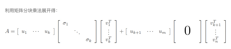
   下图中k就是r
   

$$A=XY$$

Take-away message

1. The PCA just compute Left or Right Singular Matrix (depends how you define covariance matrix) of SVD.
2. It’s unnecessary to construct a covariance matrix to start with SVD to decompose a matrix. In general, can use SGD.

Reference:
Ref1. (综合1+2)
Ref2. （1）
Ref3. （2）

One Bit Matrix Completion