


alphago网上 很多 文章写了怎么实现,一个策略网络 一个估值网络 一个蒙卡利索树,其中蒙卡利搜索树用于最后下棋的最优解运算,而策略网络 用来训练每一步的棋子该下的位置,而估值网络用于 下了棋子,运算胜出的概率。
http://renzhichu1987.blogchina.com/2917056.html 这是网上alphaGo的介绍
我们知道 训练下棋, 就是通过好多棋盘 的 棋局 作为训练的数据,来教电脑怎么下棋
我们先看看 围棋 的棋盘 19 x 19的 格子 ,上面位置地方 不是黑棋 就是 白棋 ,而如果我们把他当做一个一个像素点,那么黑子为1 白子为0 那么 他就是19x19的 二值化的灰度图片
看看输出,输出是下子的位置,如果我们把Y当做一个19x19矩阵的展开的一维向量,那么实际上每一个点的位置 [1 0 ......0]
都可以代表一个向量Y 比如 比如 [ [0,0],[1,0]] 可以flat展开成[0,0,1,0] 的一维向量
那么每一次下棋的位置 就是y的1的点,这样 每一次棋盘有多个可能的y 也就是很多的x y 对
把X 19x19图像 作为输入 Y 下棋的19x19=361长度的一维向量[0,0,0,0,0,0,0,0,0,0,0,0,0,0.....1,0,0,0,0,0,0,0] 作为Y输出来做训练。

下面我们修改网络实现我们的 alphago CNN 卷积神经网络
首先看一个AlphaGo官方开源https://github.com/Rochester-NRT/AlphaGo 但是他不是使用tensorflow而是使用 http://keras.io/ 这里我们把它使用tensorflow进行实现
这是实际使用的网络
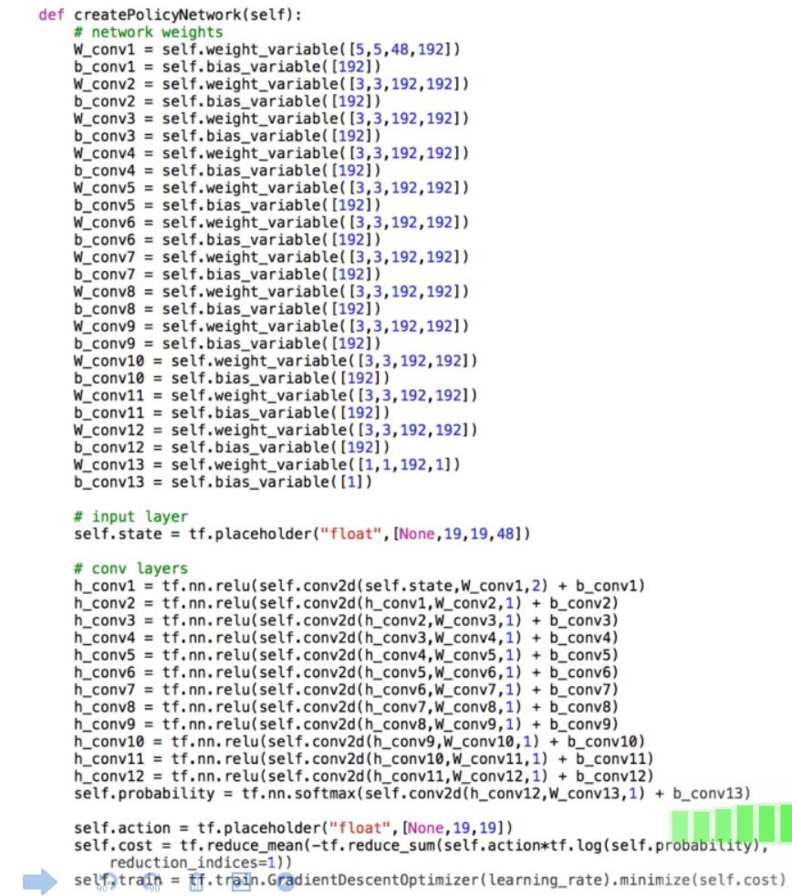
,我们这里使用自己自定义的网络、
首先贴上上一章使用的CNN模型 部分 我们只需要修改那其中的一步分就可以了
首先是X 是 19x19 的图像 ,Y值 不是0-9 的10个 而是19x19的361个
这里我们没有特别注重网络,因为网络效果 很多精度需要测试,如果要精度好,可以使用vgg16
googlenet大概有92的准确率 而resnet大概96.5的准确率,所以 后面直接修改那些网络层即可
这里看到 我们修改了输入 以及输出 以及 shape 后面调整卷积 我们卷积 层数先不调整 ,网络方面现在
现在我们计算每一步的shape
分别是
19x19 ===>21x21 ===>10x10===>12x12===>6x6===>8x8===>4x4
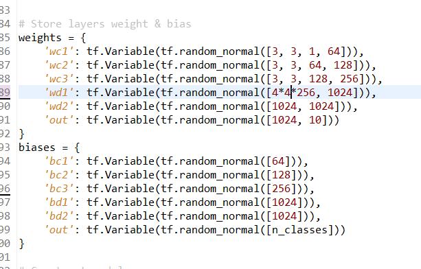
OK 我们得到了全连接层的输入 如果是用alexnet CNN来训练 alphago那么 他的输入应该是4X4X256 注意光标修改的地方
ok
我们有测试 数据来训练 ,我只讲一下 怎么使用CNN 或者我们自己自定义的CNN 来训练alphaGo的策略网络
其实我一直想的是用那些googleNet有名的CNN网络模型 来训练CNN策略网络是不是会更加智能
下面贴出修改后的代码
# Import AlphaGo Data
import input_data
mnist = input_data.read_data_sets("/tmp/data/", one_hot=True)
import tensorflow as tf
# Parameters
learning_rate = 0.001
training_iters = 200000
batch_size = 64
display_step = 20
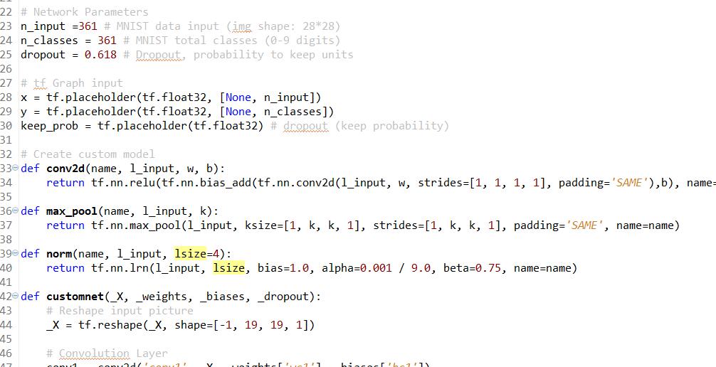
# Network Parameters
n_input =361 # alphaGo data input (img shape: 19*19)
n_classes = 361 # AlphaGo total classes (19x19=361 digits)
dropout = 0.618 # Dropout, probability to keep units 这里是随机概率当掉一些节点来训练,随你填,我一般用黄金分割点
# tf Graph input
x = tf.placeholder(tf.float32, [None, n_input])
y = tf.placeholder(tf.float32, [None, n_classes])
keep_prob = tf.placeholder(tf.float32) # dropout (keep probability)
# Create custom model
def conv2d(name, l_input, w, b):
return tf.nn.relu(tf.nn.bias_add(tf.nn.conv2d(l_input, w, strides=[1, 1, 1, 1], padding='SAME'),b), name=name)
def max_pool(name, l_input, k):
return tf.nn.max_pool(l_input, ksize=[1, k, k, 1], strides=[1, k, k, 1], padding='SAME', name=name)
def norm(name, l_input, lsize=4):
return tf.nn.lrn(l_input, lsize, bias=1.0, alpha=0.001 / 9.0, beta=0.75, name=name)
def alphago(_X, _weights, _biases, _dropout):
# Reshape input picture
_X = tf.reshape(_X, shape=[-1, 19, 19, 1])
# Convolution Layer
conv1 = conv2d('conv1', _X, _weights['wc1'], _biases['bc1'])
# Max Pooling (down-sampling)
pool1 = max_pool('pool1', conv1, k=2)
# Apply Normalization
norm1 = norm('norm1', pool1, lsize=4)
# Apply Dropout
norm1 = tf.nn.dropout(norm1, _dropout)
#conv1 image show
tf.image_summary("conv1", conv1)
# Convolution Layer
conv2 = conv2d('conv2', norm1, _weights['wc2'], _biases['bc2'])
# Max Pooling (down-sampling)
pool2 = max_pool('pool2', conv2, k=2)
# Apply Normalization
norm2 = norm('norm2', pool2, lsize=4)
# Apply Dropout
norm2 = tf.nn.dropout(norm2, _dropout)
# Convolution Layer
conv3 = conv2d('conv3', norm2, _weights['wc3'], _biases['bc3'])
# Max Pooling (down-sampling)
pool3 = max_pool('pool3', conv3, k=2)
# Apply Normalization
norm3 = norm('norm3', pool3, lsize=4)
# Apply Dropout
norm3 = tf.nn.dropout(norm3, _dropout)
# Fully connected layer
dense1 = tf.reshape(norm3, [-1, _weights['wd1'].get_shape().as_list()[0]]) # Reshape conv3 output to fit dense layer input
dense1 = tf.nn.relu(tf.matmul(dense1, _weights['wd1']) + _biases['bd1'], name='fc1') # Relu activation
dense2 = tf.nn.relu(tf.matmul(dense1, _weights['wd2']) + _biases['bd2'], name='fc2') # Relu activation
# Output, class prediction
out = tf.matmul(dense2, _weights['out']) + _biases['out']
return out
# Store layers weight & bias
weights = {
'wc1': tf.Variable(tf.random_normal([3, 3, 1, 64])),
'wc2': tf.Variable(tf.random_normal([3, 3, 64, 128])),
'wc3': tf.Variable(tf.random_normal([3, 3, 128, 256])),
'wd1': tf.Variable(tf.random_normal([4*4*256, 1024])),
'wd2': tf.Variable(tf.random_normal([1024, 1024])),
'out': tf.Variable(tf.random_normal([1024, 10]))
}
biases = {
'bc1': tf.Variable(tf.random_normal([64])),
'bc2': tf.Variable(tf.random_normal([128])),
'bc3': tf.Variable(tf.random_normal([256])),
'bd1': tf.Variable(tf.random_normal([1024])),
'bd2': tf.Variable(tf.random_normal([1024])),
'out': tf.Variable(tf.random_normal([n_classes]))
}
# Construct model
pred = customnet(x, weights, biases, keep_prob)
# Define loss and optimizer
cost = tf.reduce_mean(tf.nn.softmax_cross_entropy_with_logits(pred, y))
optimizer = tf.train.AdamOptimizer(learning_rate=learning_rate).minimize(cost)
# Evaluate model
correct_pred = tf.equal(tf.argmax(pred,1), tf.argmax(y,1))
accuracy = tf.reduce_mean(tf.cast(correct_pred, tf.float32))
# Initializing the variables
init = tf.initialize_all_variables()
#
tf.scalar_summary("loss", cost)
tf.scalar_summary("accuracy", accuracy)
# Merge all summaries to a single operator
merged_summary_op = tf.merge_all_summaries()
# Launch the graph
with tf.Session() as sess:
sess.run(init)
summary_writer = tf.train.SummaryWriter('/tmp/logs', graph_def=sess.graph_def)
step = 1
# Keep training until reach max iterations
while step * batch_size < training_iters:
batch_xs, batch_ys = mnist.train.next_batch(batch_size)
# Fit training using batch data
sess.run(optimizer, feed_dict={x: batch_xs, y: batch_ys, keep_prob: dropout})
if step % display_step == 0:
# Calculate batch accuracy
acc = sess.run(accuracy, feed_dict={x: batch_xs, y: batch_ys, keep_prob: 1.})
# Calculate batch loss
loss = sess.run(cost, feed_dict={x: batch_xs, y: batch_ys, keep_prob: 1.})
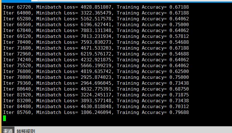
print "Iter " + str(step*batch_size) + ", Minibatch Loss= " + "{:.6f}".format(loss) + ", Training Accuracy= " + "{:.5f}".format(acc)
summary_str = sess.run(merged_summary_op, feed_dict={x: batch_xs, y: batch_ys, keep_prob: 1.})
summary_writer.add_summary(summary_str, step)
step += 1
print "Optimization Finished!"
# Calculate accuracy for 256 mnist test images
print "Testing Accuracy:", sess.run(accuracy, feed_dict={x: mnist.test.images[:256], y: mnist.test.labels[:256], keep_prob: 1.})
我没有数据,这里我就不能给大家演示截图了,但是思想方式是一样的 ,上面所有参数都是对的 。


 767
767

 被折叠的 条评论
为什么被折叠?
被折叠的 条评论
为什么被折叠?
 到【灌水乐园】发言


