Tensorflow实践之卷积神经网络模型构造、保存和读取

Tensorflow实践之卷积神经网络模型构造、保存和读取

本次实验是在Jupyter上进行，训练集下载地址为：https://www.kaggle.com/moltean/fruits
1.图像采集与预处理

##导包
import os
import skimage
import numpy as np
import matplotlib.pyplot as plt
from skimage import color,data,transform
from sklearn.utils import shuffle
import keras
from keras.utils import np_utils
import skimage.io
os.chdir('训练集文件夹所在目录')

采集数据

##由于数据集过大,先加载小部分进行训练，m代表几个类
def load_small_data(dir_path,m):
    images_m=[] ##新建一个空列表用于存放图片数集
    labels_m=[] ##新建一个空列表用于存放标签数集
    lab=os.listdir(dir_path)
    n=0
    for l in lab:
        if(n>=m):
            break
        img=os.listdir(dir_path+l) ##img为对应路径下的文件夹
        for i in img:
            img_path=dir_path+l+'/'+i ##是的话获取图片路径
            labels_m.append(int(n)) ##将图片的上层文件夹转换为int类型存于labels中
            images_m.append(skimage.io.imread(img_path)) ##读取对应路径图像存放于images_m中
        n+=1
    return images_m,labels_m ## m类标签以及数据

获得训练集和测试集

images_10,labels_10=load_small_data('./Training/',10) ##训练集
images_test_10,labels_test_10=load_small_data('./Test/',10) ##测试集

对图像进行预处理

##使用列表推导式完成图像的批量裁剪
def cut_image(images,w,h):
    new_images=[skimage.transform.resize(I,(w,h)) for I in images]
    return new_images
##预处理数据函数（数组化，乱序）
def prepare_data(images,labels,n_classes):
    images64=cut_image(images,100,100) ##裁剪图片大小为100*100
    train_x=np.array(images)
    train_y=np.array(labels)
    ##images_gray=color.rgb2gray(images_a) ##转灰度
    indx=np.arange(0,train_y.shape[0])
    indx=shuffle(indx)
    train_x=train_x[indx]
    train_y=train_y[indx]
    train_y=keras.utils.to_categorical(train_y,n_classes) ##one-hot独热编码
    return train_x,train_y

##训练集数据预处理
train_x,train_y=prepare_data(images_10,labels_10,10)
##测试数据集与标签的数组化和乱序
test_x,test_y=prepare_data(images_test_10,labels_test_10,10)

2.构建卷积神经网络
本实验采用经典模型LeNet-5模型搭建的两层卷积池化，三层全连实现。LeNet-5是经典的卷积神经网络之一，LeNet包含两个卷积层，2个全连接层，共计6万个学习参数。

import tensorflow as tf
## 配置神经网络的参数
n_classes=10 ##数据的类别数
batch_size=128 ##训练块的大小
kernel_h=kernel_w=5 ##卷积核尺寸
dropout=0.8 ##dropout的概率
depth_in=3 ##图片的通道数
depth_out1=64 ##第一层卷积的卷积核个数
depth_out2=128 ##第二层卷积的卷积核个数
image_size=train_x.shape[1] ##图片尺寸
n_sample=train_x.shape[0] ##训练样本个数
t_sample=test_x.shape[0] ##测试样本个数
 
##feed给神经网络的图像数据类型与shape,四维，第一维训练的数据量，第二、三维图片尺寸，第四维图像通道数
with tf.name_scope('input'): 
    x=tf.placeholder(tf.float32,[None,100,100,3], name='x') 
    y=tf.placeholder(tf.float32,[None,n_classes], name='y') ##feed到神经网络的标签数据的类型和shape
keep_prob=tf.placeholder(tf.float32) ##dropout的placeholder(解决过拟合)
fla=int((image_size*image_size/16)*depth_out2) ##用于扁平化处理的参数经过两层卷积池化后的图像大小*第二层的卷积核个数
##定义各卷积层和全连接层的权重变量
Weights={"con1_w":tf.Variable(tf.random_normal([kernel_h,kernel_w,depth_in,depth_out1])),\
        "con2_w":tf.Variable(tf.random_normal([kernel_h,kernel_w,depth_out1,depth_out2])),\
        "fc_w1":tf.Variable(tf.random_normal([int((image_size*image_size/16)*depth_out2),1024])),\
        "fc_w2":tf.Variable(tf.random_normal([1024,512])),\
        "out":tf.Variable(tf.random_normal([512,n_classes]))}
 
##定义各卷积层和全连接层的偏置变量
bias={"conv1_b":tf.Variable(tf.random_normal([depth_out1])),\
      "conv2_b":tf.Variable(tf.random_normal([depth_out2])),\
      "fc_b1":tf.Variable(tf.random_normal([1024])),\
      "fc_b2":tf.Variable(tf.random_normal([512])),\
      "out":tf.Variable(tf.random_normal([n_classes]))}
## 定义卷积层的生成函数
def conv2d(x,W,b,stride=1):
    x=tf.nn.conv2d(x,W,strides=[1,stride,stride,1],padding="SAME")
    x=tf.nn.bias_add(x,b)
    return tf.nn.relu(x)
 
## 定义池化层的生成函数
def maxpool2d(x,stride=2):
    return tf.nn.max_pool(x,ksize=[1,stride,stride,1],strides=[1,stride,stride,1],padding="SAME")
 
## 定义卷积神经网络生成函数
def conv_net(x,weights,biases,dropout):
    
    ## Convolutional layer 1(卷积层1)
    conv1 = conv2d(x,Weights['con1_w'],bias['conv1_b']) ##100*100*64
    conv1 = maxpool2d(conv1,2) ##经过池化层1 shape：50*50*64
     
    ## Convolutional layer 2（卷积层2）
    conv2 = conv2d(conv1,Weights['con2_w'],bias['conv2_b']) ##50*50*128
    conv2 = maxpool2d(conv2,2) ##经过池化层2 shape:25*25*128
    ## Fully connected layer 1(全连接层1)
    flatten = tf.reshape(conv2,[-1,fla]) ##Flatten层，扁平化处理
    fc1 = tf.add(tf.matmul(flatten,Weights['fc_w1']),bias['fc_b1'])
    fc1 = tf.nn.relu(fc1) ##经过relu激活函数
    print(flatten.get_shape())
    ## Fully connected layer 2(全连接层2)
    fc2 = tf.add(tf.matmul(fc1,Weights['fc_w2']),bias['fc_b2']) ##计算公式：输出参数=输入参数*权值+偏置
    fc2 = tf.nn.relu(fc2) ##经过relu激活函数
    
    ## Dropout（Dropout层防止预测数据过拟合）
    fc2 = tf.nn.dropout(fc2,dropout)
    ## Output class prediction
    prediction = tf.add(tf.matmul(fc2,Weights['out']),bias['out']) ##输出预测参数
    return prediction      

3.选择优化器
人工神经网络是由很多神经元组成的，每个神经元都有自己的权重w，表示在某项任务中，该神经元的重要程度。假设输入数据为x，那么预测值即为：prediction = wx + b 为获得最佳的训练效果，计算合适的w和b即 使 loss （sum(|(y_ - prediction)|)） 尽可能小。优化器（optimizer）就是对w和b参数的调节，以找到最优解。

## 优化预测准确率
with tf.name_scope('prediction'):
    prediction=conv_net(x,Weights,bias,keep_prob) ##生成卷积神经网络
    b = tf.constant(value=1,dtype=tf.float32)
    prediction_eval = tf.multiply(prediction,b,name='prediction_eval') 
cross_entropy=tf.reduce_mean(tf.nn.softmax_cross_entropy_with_logits_v2(logits=prediction,labels=y)) ##交叉熵损失函数
optimizer=tf.train.AdamOptimizer(0.0009).minimize(cross_entropy) ##选择优化器以及学习率

##optimizer=tf.train.GradientDescentOptimizer(0.1).minimize(cross_entropy)
##optimizer=tf.train.AdagradOptimizer(0.001).minimize(cross_entropy) ##选择优化器以及学习率
 
## 评估模型
with tf.name_scope('accuracy'):
    correct_pred=tf.equal(tf.argmax(prediction,1),tf.argmax(y,1))
    accuracy=tf.reduce_mean(tf.cast(correct_pred,tf.float32),name='accuracy')

这里会出现一个警告不过不影响结果
4.开始训练数据并保存模型

##训练块数据生成器
def gen_small_data(inputs,batch_size):
    i=0
    while True:
        small_data=inputs[i:(batch_size+i)]
        i+=batch_size
        yield small_data

# 初始会话并开始训练过程
with tf.Session() as sess:
    tf.global_variables_initializer().run()   
    for  i  in range(7):
        train_x,train_y=prepare_data(images_10,labels_10,10) ##重新预处理数据
        train_x=gen_small_data(train_x,batch_size) ##生成图像块数据
        train_y=gen_small_data(train_y,batch_size) ##生成标签块数据
        for j in range(10):
            x_=next(train_x) 
            y_=next(train_y)
            ##准备验证数据
            validate_feed={x:x_,y:y_,keep_prob:0.8}
            sess.run(optimizer, feed_dict=validate_feed)
            loss,acc = sess.run([cross_entropy,accuracy],feed_dict={x:x_,y:y_,keep_prob:0.8})
            print("Epoch:", '%04d' % i,"cost=", "{:.9f}".format(loss),"Training accuracy","{:.5f}".format(acc))
            i=i+1
    print('Optimization Completed')
    ##准备测试数据
    test_x=test_x[0:400]
    test_y=test_y[0:400]
    test_feed={x:test_x,y:test_y,keep_prob: 0.8}
    saver = tf.train.Saver()
    y1 = sess.run(prediction,feed_dict=test_feed)
    for epoch in range(11):##保存模型
        if epoch % 10 == 0:
            print ("------------------------------------------------------")
            saver.save(sess,"模型保存地址",global_step=epoch)
            print("save the model")
            test_classes = np.argmax(y1,1)
            print('Testing Accuracy:',sess.run(accuracy,feed_dict=test_feed))
print ("------------------------------------------------------")

训练过程

保存完成的模型如下图所示：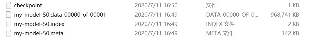

5.利用模型进行水果识别

import os
os.environ['TF_CPP_MIN_LOG_LEVEL'] = '2'

from skimage import io,transform
import tensorflow as tf
import numpy as np


path1 = "待测图片文件夹/1.jpg"
path2 = "待测图片文件夹/2.jpg"
path3 = "待测图片文件夹/3.jpg"
path4 = "待测图片文件夹/4.jpg"
path5 = "待测图片文件夹/5.jpg"
path6 = "待测图片文件夹/6.jpg"
path7 = "待测图片文件夹/7.jpg"
path8 = "待测图片文件夹/8.jpg"
path9 = "待测图片文件夹/9.jpg"
path10 = "待测图片文件夹/10.jpg"


flower_dict = {0:'Apple',1:'Banana',2:'Banana Red',3:'Blueberry',4:'Clementine',
               5:'Lemon',6:'Lychee',7:'Mulberry',8:'Orange',9:'Peach'}

w=100
h=100
c=3

def read_one_image(path):
    img = io.imread(path)
    img = transform.resize(img,(w,h))
    return np.asarray(img)

with tf.Session() as sess:
    data = []
    data1 = read_one_image(path1)
    data2 = read_one_image(path2)
    data3 = read_one_image(path3)
    data4 = read_one_image(path4)
    data5 = read_one_image(path5)
    data6 = read_one_image(path6)
    data7 = read_one_image(path7)
    data8 = read_one_image(path8)
    data9 = read_one_image(path9)
    data10 = read_one_image(path10)

    data.append(data1)
    data.append(data2)
    data.append(data3)
    data.append(data4)
    data.append(data5)
    data.append(data6)
    data.append(data7)
    data.append(data8)
    data.append(data9)
    data.append(data10)


    saver = tf.train.import_meta_graph('模型中.meta文件所在目录')
    saver.restore(sess,tf.train.latest_checkpoint('模型所在文件夹以/结尾'))

    graph = tf.get_default_graph()
    x = graph.get_tensor_by_name("input/x:0")
    feed_dict = {x:data,keep_prob: 0.8}

    prediction = graph.get_tensor_by_name("prediction/prediction_eval:0")

    classification_result = sess.run(prediction,feed_dict)

    #打印出预测矩阵
    print(classification_result)
    #打印出预测矩阵每一行最大值的索引
    print(tf.argmax(classification_result,1).eval())
    #根据索引通过字典对应花的分类
    output = []
    output = tf.argmax(classification_result,1).eval()
    for i in range(len(output)):
        print("第",i+1,"种水果预测:"+flower_dict[output[i]])

预测结果：

6.水果识别结果可视化

import matplotlib.pyplot as plt
import numpy as np
def plot_images_labels_prediction(images,prediction,idx,num=10):
    fig = plt.gcf()
    fig.set_size_inches(10, 12)
    if num>25: 
        num=25 
    for i in range(0,num):
        ax=plt.subplot(5,5, 1+i)
        
        ax.imshow(np.reshape(images[idx],(100, 100,3)))
        if len(prediction)>0:
            title="predict="+str(flower_dict[prediction[idx]])

            
        ax.set_title(title,fontsize=10) 
        ax.set_xticks([]);ax.set_yticks([])        
        idx+=1 
    plt.show()

%matplotlib inline

plot_images_labels_prediction(data,output,0)

结果如下图所示：