


首先对于模型: SARIMA(p,d,q)x(P,D,Q)。
参数的选择的注意事项如下:
where, P, D and Q are SAR, order of seasonal differencing and SMA terms respectively and ‘x’ is the frequency of the time series. If the model has well defined seasonal patterns, then enforce D=1 for a given frequency ‘x’.
We should set the model parameters such that D never exceeds one. And the total differencing ‘d + D’ never exceeds 2. We should try to keep only either SAR or SMA terms if the model has seasonal components.
代码如下:
# 导入必要的包
import matplotlib.pyplot as plt
import pandas as pd
# 数据读入
time_series_table=pd.read_csv('new_merged.csv',index_col=0,parse_dates=True)
time_series_table=time_series_table.sort_index()
print(time_series_table)
from statsmodels.tsa.statespace.sarimax import SARIMAX

# 季节模型的拟合
best_model = SARIMAX(time_series_table['33_1002'][:-432], order=(0, 0, 2), seasonal_order=(0, 1, 2, 144)).fit(dis=-1)
best_model.summary()
%%time
# 模型拟合情况检查
best_model.plot_diagnostics(figsize=(15,12));
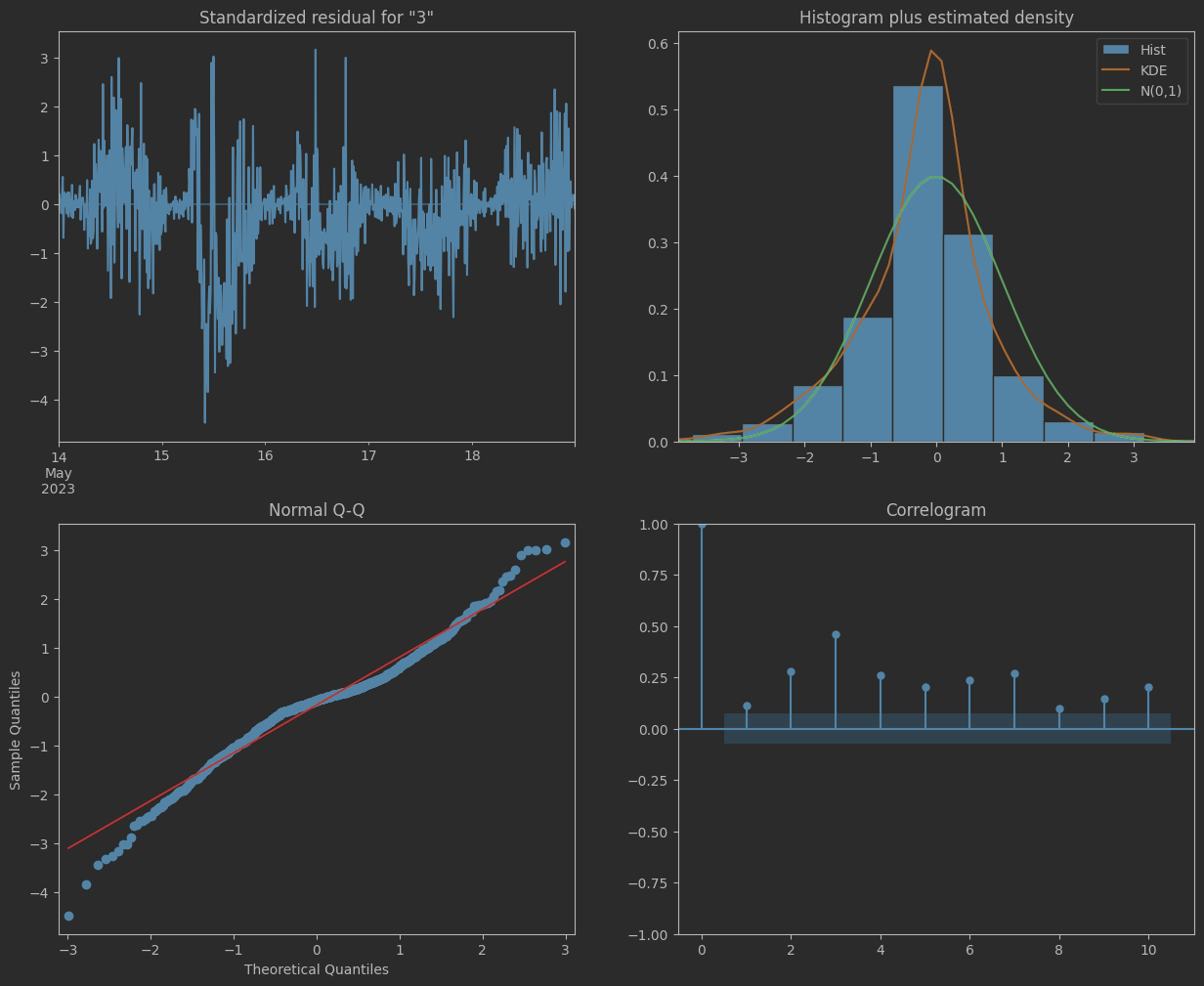
这里的检查主要是考虑了季节拟合之后的残差的检查。
下面检查是否需要季节差分。
# Plot
data=time_series_table["21_1002"]

fig, axes = plt.subplots(2, 1, figsize=(10,5), dpi=100, sharex=True)

# Usual Differencing
axes[0].plot(data[:], label='Original Series')
axes[0].plot(data[:].diff(1), label='Usual Differencing')
axes[0].set_title('Usual Differencing')
axes[0].legend(loc='upper left', fontsize=10)


# Seasonal Differencing
axes[1].plot(data[:], label='Original Series')
axes[1].plot(data[:].diff(144), label='Seasonal Differencing', color='green')
axes[1].set_title('Seasonal Differencing')
plt.legend(loc='upper left', fontsize=10)
plt.suptitle('Drug Sales - Time Series Dataset', fontsize=16)
plt.show()
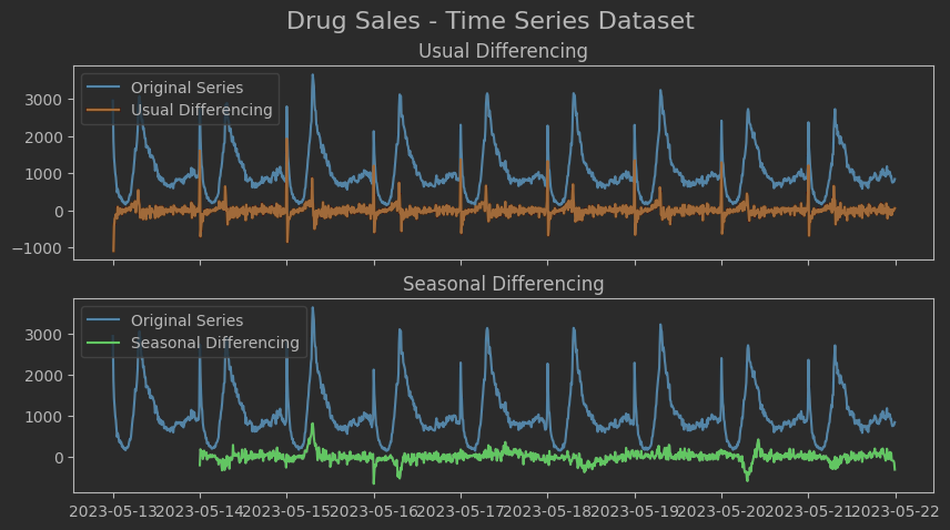
差分之后的绿色线条显示序列比较平稳。
target="33_1002"
# 定义测试集和训练集如何分割
train_start_dt = '2023-05-14 00:00:00'
test_start_dt = '2023-05-19 00:00:00'
train = time_series_table.copy()[(time_series_table.index >= train_start_dt) & (time_series_table.index < test_start_dt)][[target]]
test = time_series_table.copy()[time_series_table.index >= test_start_dt][[target]]
pred = best_model.predict(start=test.index[0], end=test.index[-1])
利用mape指标对拟合的效果进行评估。
import numpy as np

# 分析 mape 的函数如下
def analysis(predict,test):

    def mape(predictions, actuals):
        """Mean absolute percentage error"""
        predictions = np.array(predictions)
        actuals = np.array(actuals)
        return (np.absolute(predictions - actuals) / actuals).mean()

    mape1=  mape(predict, test)
    mape2=  mape(test.shift(1).dropna(), test[1:])

    print('predict-actual MAPE: ', mape1 * 100, '%')
    print('shifted1-actual MAPE: ', mape2 * 100, '%')
    print('mape improvement',(mape1-mape2)/mape2)
Github上一个很好的例子:
github.com/marcopeix/time-series-analysis/blob/master/Advanced%20modelling/SARIMA.ipynb
总结:季节 SARIMAX 不适合把周期指定的很大,这里指定为144,拟合的速度非常慢, 并且吃内存。
best_model = SARIMAX(time_series_table['33_1002'][:-432], order=(0, 0, 2), seasonal_order=(0, 1, 2, 144)).fit(dis=-1)


 2万+
2万+


 被折叠的 条评论
为什么被折叠?
被折叠的 条评论
为什么被折叠?
 到【灌水乐园】发言


