


文章目录
环境
- python 3.8
- tensorflow 2.3.0
1 准备数据
使用 Max Planck Institute for Biogeochemistry 的天气时间序列数据集。
该数据集包含14个不同的特征,例如气温,大气压力和湿度。从2003年开始,每10分钟收集一次。为了提高效率,本文仅使用2009年至2016年之间收集的数据。
导入需要的库
#导入需要的库
import tensorflow as tf
import matplotlib as mpl
import matplotlib.pyplot as plt
import numpy as np
import os
import pandas as pd

mpl.rcParams['figure.figsize'] = (8, 6)
mpl.rcParams['figure.dpi'] = 150
mpl.rcParams['axes.grid'] = False
导入数据
zip_path = tf.keras.utils.get_file(
	origin='https://storage.googleapis.com/tensorflow/tf-keras-			datasets/jena_climate_2009_2016.csv.zip',
    fname='jena_climate_2009_2016.csv.zip',
    extract=True)
csv_path, _ = os.path.splitext(zip_path)
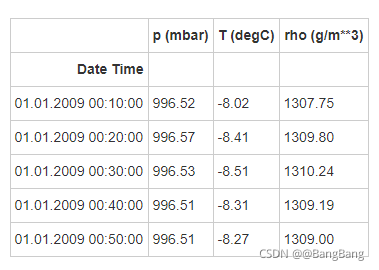
df = pd.read_csv(csv_path)
df.head()
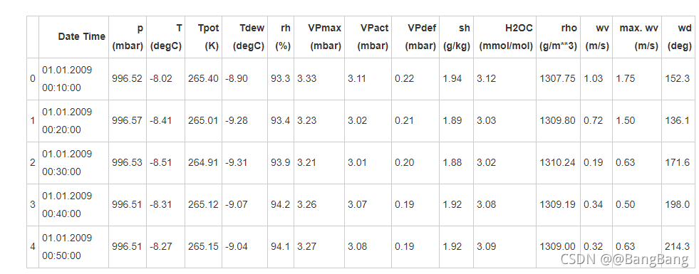
如上所示,每10分钟记录一次观测值,一个小时内有6个观测值,一天有144(6x24)个观测值。
给定一个特定的时间,假设要预测未来6小时的温度。为了做出此预测,选择使用5天的观察时间。因此,创建一个包含最后720(5x144)个观测值的窗口以训练模型。
下面的函数返回上述时间窗以供模型训练。参数history_size 是过去信息的滑动窗口大小。target_size 是模型需要学习预测的未来时间步,也作为需要被预测的标签。
下面使用数据的前300,000行当做训练数据集,其余的作为验证数据集。总计约2100天的训练数据。
划分训练特征和标签
def univariate_data(dataset, start_index, end_index, history_size, target_size):
    data = []
    labels = []

    start_index = start_index + history_size
    if end_index is None:
        end_index = len(dataset) - target_size

    for i in range(start_index, end_index):
        indices = range(i-history_size, i)
        # Reshape data from (history`1_size,) to (history_size, 1)
        data.append(np.reshape(dataset[indices], (history_size, 1)))
        labels.append(dataset[i+target_size])
    return np.array(data), np.array(labels)
for i in range(0,10):
    indices = range(i-20, i)
    print(indices)
range(-20, 0)
range(-19, 1)
range(-18, 2)
range(-17, 3)
range(-16, 4)
range(-15, 5)
range(-14, 6)
range(-13, 7)
range(-12, 8)
range(-11, 9)
参数设置
TRAIN_SPLIT = 300000
# 设置种子以确保可重复性。
tf.random.set_seed(13)
2 单变量单步
首先,使用一个特征(温度)训练模型,并在使用该模型做预测。
从数据集中提取温度
uni_data = df['T (degC)']
uni_data.index = df['Date Time']
uni_data.head()
Date Time
01.01.2009 00:10:00   -8.02
01.01.2009 00:20:00   -8.41
01.01.2009 00:30:00   -8.51
01.01.2009 00:40:00   -8.31
01.01.2009 00:50:00   -8.27
Name: T (degC), dtype: float64
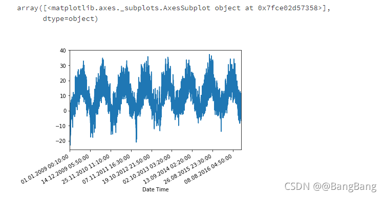
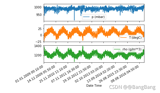
观察数据随时间变化的情况
uni_data.plot(subplots=True)
#将数据集转换为数组类型
uni_data = uni_data.values
uni_data
标准化
#标准化
uni_train_mean = uni_data[:TRAIN_SPLIT].mean()
uni_train_std = uni_data[:TRAIN_SPLIT].std()

uni_data = (uni_data-uni_train_mean)/uni_train_std
用前history_size个时间点的温度预测第history_size+target_size+1个时间点的温度。start_index和end_index表示数据集datasets起始的时间点,我们将要从这些时间点中取出特征和标签。
每个样本有20个特征(即20个时间点的温度信息),其标签为第21个时间点的温度值,如:
#写函数来划分特征和标签
univariate_past_history = 20
univariate_future_target = 0
x_train_uni, y_train_uni = univariate_data(uni_data, 0, TRAIN_SPLIT, # 起止区间
                                           univariate_past_history,
                                           univariate_future_target)
x_val_uni, y_val_uni = univariate_data(uni_data, TRAIN_SPLIT, None,
                                       univariate_past_history,
                                       univariate_future_target)
可见第一个样本的特征为前20个时间点的温度,其标签为第21个时间点的温度。根据同样的规律,第二个样本的特征为第2个时间点的温度值到第21个时间点的温度值,其标签为第22个时间点的温度……
x_train_uni.shape
>> (299980, 20, 1)
y_train_uni.shape
>> (299980,)
x_val_uni.shape
>> (120531, 20, 1)
print ('Single window of past history')
print (x_train_uni[0])
print ('\n Target temperature to predict')
print (y_train_uni[0])
Single window of past history
[[-1.99766294]
 [-2.04281897]
 [-2.05439744]
 [-2.0312405 ]
 [-2.02660912]
 [-2.00113649]
 [-1.95134907]
 [-1.95134907]
 [-1.98492663]
 [-2.04513467]
 [-2.08334362]
 [-2.09723778]
 [-2.09376424]
 [-2.09144854]
 [-2.07176515]
 [-2.07176515]
 [-2.07639653]
 [-2.08913285]
 [-2.09260639]
 [-2.10418486]]

 Target temperature to predict
-2.1041848598100876
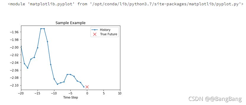
设置绘图函数
def create_time_steps(length):
    return list(range(-length, 0))

def show_plot(plot_data, delta, title):
    labels = ['History', 'True Future', 'Model Prediction']
    marker = ['.-', 'rx', 'go']
    time_steps = create_time_steps(plot_data[0].shape[0]) # 横轴刻度
    if delta:
        future = delta
    else:
        future = 0

    plt.title(title)
    for i, x in enumerate(plot_data):
        if i:
            plt.plot(future, plot_data[i], marker[i], markersize=10,
                     label=labels[i])
        else:
            plt.plot(time_steps, plot_data[i].flatten(), marker[i], label=labels[i])
    plt.legend()
    plt.xlim([time_steps[0], (future+5)*2])
    plt.xlabel('Time-Step')
    return plt
show_plot([x_train_uni[0], y_train_uni[0]], 0, 'Sample Example')
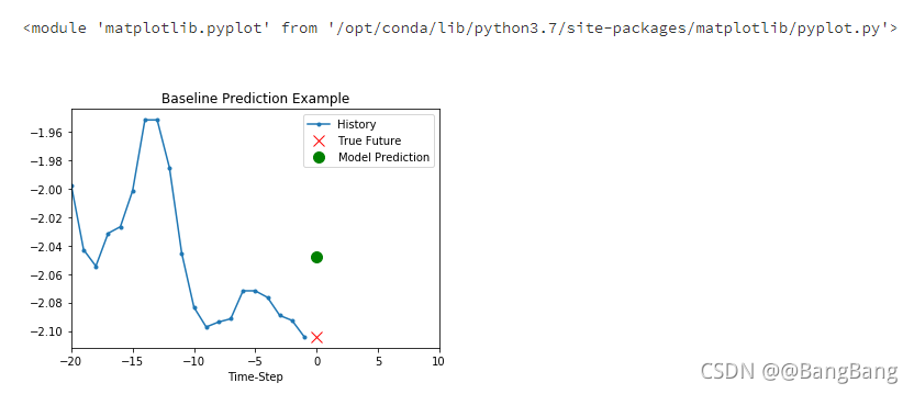
def baseline(history):
    return np.mean(history)

show_plot([x_train_uni[0], y_train_uni[0], baseline(x_train_uni[0])], 0,
           'Baseline Prediction Example')
将特征和标签切片
BATCH_SIZE = 256
BUFFER_SIZE = 10000

train_univariate = tf.data.Dataset.from_tensor_slices((x_train_uni, y_train_uni))
train_univariate = train_univariate.cache().shuffle(BUFFER_SIZE).batch(BATCH_SIZE).repeat()

val_univariate = tf.data.Dataset.from_tensor_slices((x_val_uni, y_val_uni))
val_univariate = val_univariate.batch(BATCH_SIZE).repeat()
建模
simple_lstm_model = tf.keras.models.Sequential([
    tf.keras.layers.LSTM(8, input_shape=x_train_uni.shape[-2:]), # input_shape=(20,1) 不包含批处理维度
    tf.keras.layers.Dense(1)
])

simple_lstm_model.compile(optimizer='adam', loss='mae')
训练模型
EVALUATION_INTERVAL = 200
EPOCHS = 10

simple_lstm_model.fit(train_univariate, epochs=EPOCHS,
                      steps_per_epoch=EVALUATION_INTERVAL,
                      validation_data=val_univariate, validation_steps=50)
Train for 200 steps, validate for 50 steps
Epoch 1/10
200/200 [==============================] - 5s 27ms/step - loss: 0.4075 - val_loss: 0.1351
Epoch 2/10
200/200 [==============================] - 4s 19ms/step - loss: 0.1118 - val_loss: 0.0359
Epoch 3/10
200/200 [==============================] - 4s 19ms/step - loss: 0.0489 - val_loss: 0.0290
Epoch 4/10
200/200 [==============================] - 4s 19ms/step - loss: 0.0443 - val_loss: 0.0258
Epoch 5/10
200/200 [==============================] - 4s 19ms/step - loss: 0.0299 - val_loss: 0.0235
Epoch 6/10
200/200 [==============================] - 4s 19ms/step - loss: 0.0317 - val_loss: 0.0224
Epoch 7/10
200/200 [==============================] - 4s 19ms/step - loss: 0.0286 - val_loss: 0.0208
Epoch 8/10
200/200 [==============================] - 4s 19ms/step - loss: 0.0263 - val_loss: 0.0200
Epoch 9/10
200/200 [==============================] - 4s 19ms/step - loss: 0.0254 - val_loss: 0.0182
Epoch 10/10
200/200 [==============================] - 4s 20ms/step - loss: 0.0228 - val_loss: 0.0174
print(val_univariate)
print(val_univariate.take(3))
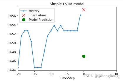
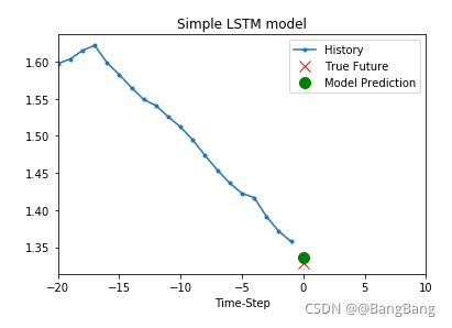
for x, y in val_univariate.take(3):
    plot = show_plot([x[0].numpy(), y[0].numpy(),simple_lstm_model.predict(x)[0]], 0, 'Simple LSTM model')
    plot.show()

3 多变量单步
在这里,我们用过去的一些压强信息、温度信息以及密度信息来预测未来的一个时间点的温度。也就是说,数据集中应该包括压强信息、温度信息以及密度信息。
从数据集中划分特征和标签
features_considered = ['p (mbar)', 'T (degC)', 'rho (g/m**3)']
features = df[features_considered]
features.index = df['Date Time']
features.head()
压强、温度、密度随时间变化绘图
features.plot(subplots=True)
将数据集转换为数组类型并标准化
dataset = features.values
data_mean = dataset[:TRAIN_SPLIT].mean(axis=0)
data_std = dataset[:TRAIN_SPLIT].std(axis=0)

dataset = (dataset-data_mean)/data_std
写函数来划分特征和标签
在这里,我们不再像单变量单步中一样用到每个数据,而是在函数中加入step参数,这表明所使用的样本每step个时间点取一次特征和标签。
def multivariate_data(dataset, target, start_index, end_index, history_size,
                      target_size, step, single_step=False):
    data = []
    labels = []

    start_index = start_index + history_size

    if end_index is None:
        end_index = len(dataset) - target_size

    for i in range(start_index, end_index):
        indices = range(i-history_size, i, step) # step表示滑动步长
        data.append(dataset[indices])

        if single_step:
            labels.append(target[i+target_size])
        else:
            labels.append(target[i:i+target_size])

    return np.array(data), np.array(labels)
past_history = 720
future_target = 72
STEP = 6

x_train_single, y_train_single = multivariate_data(dataset, dataset[:, 1], 0,
                                                   TRAIN_SPLIT, past_history,
                                                   future_target, STEP,
                                                   single_step=True)
x_val_single, y_val_single = multivariate_data(dataset, dataset[:, 1],
                                               TRAIN_SPLIT, None, past_history,
                                               future_target, STEP,
                                               single_step=True)
将特征和标签切片
train_data_single = tf.data.Dataset.from_tensor_slices((x_train_single, y_train_single))
train_data_single = train_data_single.cache().shuffle(BUFFER_SIZE).batch(BATCH_SIZE).repeat()

val_data_single = tf.data.Dataset.from_tensor_slices((x_val_single, y_val_single))
val_data_single = val_data_single.batch(BATCH_SIZE).repeat()
建模
single_step_model = tf.keras.models.Sequential()
single_step_model.add(tf.keras.layers.LSTM(32,
                                           input_shape=x_train_single.shape[-2:]))
single_step_model.add(tf.keras.layers.Dense(1))

single_step_model.compile(optimizer=tf.keras.optimizers.RMSprop(), loss='mae')

single_step_history = single_step_model.fit(train_data_single, epochs=EPOCHS,
                                            steps_per_epoch=EVALUATION_INTERVAL,
                                            validation_data=val_data_single,
                                            validation_steps=50)
Train for 200 steps, validate for 50 steps
Epoch 1/10
200/200 [==============================] - 31s 155ms/step - loss: 0.3090 - val_loss: 0.2647
Epoch 2/10
200/200 [==============================] - 29s 144ms/step - loss: 0.2623 - val_loss: 0.2444
Epoch 3/10
200/200 [==============================] - 30s 148ms/step - loss: 0.2612 - val_loss: 0.2460
Epoch 4/10
200/200 [==============================] - 31s 157ms/step - loss: 0.2567 - val_loss: 0.2440
Epoch 5/10
200/200 [==============================] - 32s 158ms/step - loss: 0.2263 - val_loss: 0.2362
Epoch 6/10
200/200 [==============================] - 31s 156ms/step - loss: 0.2413 - val_loss: 0.2659
Epoch 7/10
200/200 [==============================] - 30s 149ms/step - loss: 0.2415 - val_loss: 0.2572
Epoch 8/10
200/200 [==============================] - 30s 148ms/step - loss: 0.2410 - val_loss: 0.2380
Epoch 9/10
200/200 [==============================] - 30s 148ms/step - loss: 0.2445 - val_loss: 0.2490
Epoch 10/10
200/200 [==============================] - 30s 149ms/step - loss: 0.2390 - val_loss: 0.2479
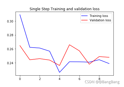
def plot_train_history(history, title):
    loss = history.history['loss']
    val_loss = history.history['val_loss']

    epochs = range(len(loss))

    plt.figure()

    plt.plot(epochs, loss, 'b', label='Training loss')
    plt.plot(epochs, val_loss, 'r', label='Validation loss')
    plt.title(title)
    plt.legend()

    plt.show()
训练模型
plot_train_history(single_step_history,
                   'Single Step Training and validation loss')
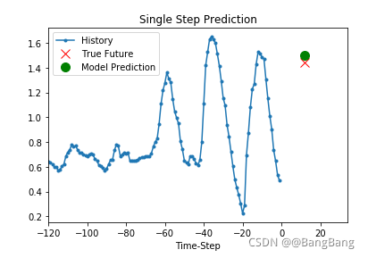
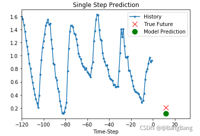
绘制预测图
for x, y in val_data_single.take(3):
    plot = show_plot([x[0][:, 1].numpy(), y[0].numpy(),
                    single_step_model.predict(x)[0]], 12,
                   'Single Step Prediction')
    plot.show()

4 多变量多步
从数据集中划分特征和标签
future_target = 72
x_train_multi, y_train_multi = multivariate_data(dataset, dataset[:, 1], 0,
                                                 TRAIN_SPLIT, past_history,
                                                 future_target, STEP)
x_val_multi, y_val_multi = multivariate_data(dataset, dataset[:, 1],
                                             TRAIN_SPLIT, None, past_history,
                                             future_target, STEP)
将特征和标签切片
train_data_multi = tf.data.Dataset.from_tensor_slices((x_train_multi, y_train_multi))
train_data_multi = train_data_multi.cache().shuffle(BUFFER_SIZE).batch(BATCH_SIZE).repeat()

val_data_multi = tf.data.Dataset.from_tensor_slices((x_val_multi, y_val_multi))
val_data_multi = val_data_multi.batch(BATCH_SIZE).repeat()
编写绘图函数
def multi_step_plot(history, true_future, prediction):
    plt.figure(figsize=(12, 6))
    num_in = create_time_steps(len(history))
    num_out = len(true_future)

    plt.plot(num_in, np.array(history[:, 1]), label='History')
    plt.plot(np.arange(num_out)/STEP, np.array(true_future), 'bo',
           label='True Future')
    if prediction.any():
        plt.plot(np.arange(num_out)/STEP, np.array(prediction), 'ro',
                 label='Predicted Future')
    plt.legend(loc='upper left')
    plt.show()
for x, y in train_data_multi.take(1):
    multi_step_plot(x[0], y[0], np.array([0]))
建模
multi_step_model = tf.keras.models.Sequential()
multi_step_model.add(tf.keras.layers.LSTM(32,
                                          return_sequences=True,
                                          input_shape=x_train_multi.shape[-2:]))
multi_step_model.add(tf.keras.layers.LSTM(16, activation='relu'))
multi_step_model.add(tf.keras.layers.Dense(72))

multi_step_model.compile(optimizer=tf.keras.optimizers.RMSprop(clipvalue=1.0), loss='mae')
训练模型
multi_step_history = multi_step_model.fit(train_data_multi, epochs=EPOCHS,
                                          steps_per_epoch=EVALUATION_INTERVAL,
                                          validation_data=val_data_multi,
                                          validation_steps=50)
plot_train_history(multi_step_history, 'Multi-Step Training and validation loss')
绘制温度信息
for x, y in val_data_multi.take(3):
    multi_step_plot(x[0], y[0], multi_step_model.predict(x)[0])
5 模型保存
保存为.pb格式文件
mutli_step_model.save('mutli_tempter','/model_save_path')
print('模型已保存')
就是这么简单,保存之后会在 model_save_path 下生成如下三个文件。

pb模型的加载
mutli_step_model=tf.keras.models.load_model(".\model_save_path")
保存为.h5格式文件
mutli_step_model.save('mutli_tempter.h5')
print('模型已保存')
h5模型的加载
mutli_step_model=tf.keras.models.load_model("mutli_tempter.h5")
6 转换为TFLite模型
tflite 模型转换
run_model=tf.function(lambda x:multi_step_model(x))
# This is import,let's fix the input size (需要固定模型输入的大小,不然调用tflite模型会报错:"Error:size should be keep static not dynamic")
BATCH_SIZE=1
STEPS=120
INPUT_SIZE=3

concrete_func=run_model.get_concrete_function(
		tf.TensorSpec([BATCH_SIZE,STEPS,INPUT_SIZE],multi_step_model.inputs[0].dtype)
)

#model directory
MODEL_DIR="keras_lstm"
multi_step_model.save(MODEL_DIR,save_format="tf",signatures=concrete_func)

converter=tf.lite.TFLiteConverter.from_saved_model(MODEL_DIR)
tflite_model=converter.convert()
open('multi_tempter.tflite','wb').write(tflite_model)
print('saved tflite model!')
验证python 调取tflite模型
Now load TensorFlow Lite model and use the Tensorflow Lite python interpreter to verify the results
# Run the model with Tensorflow to get expected results
TEST_CASES = 10

#Run the model with Tensorflow Lite
interpreter=tf.lite.Interpreter(model_content=tflite_model)
interpreter.allocate_tensors()
input_details=interpreter.get_input_details()
output_details=interpreter.get_output_details()

print("input_details",input_details)
print("output_details",output_details)

for i in range(TEST_CASES):
	expected=mutli_step_model.predict(x_val_multi[i:i+1])
	interpreter.set_tensor(input_details[0]["index"],x_val_multi[i:i+1,:,:].astype(np.float32))
	interpreter.invoke()
	result=interpreter.get_tensor(output_details[0]["index"])

	#Assert if the result of TFLite model is consistent with the tf model
	np.testing.assert_almost_equal(expected,result)
	print("Down.The reuslt of Tensorflow matches the result of Tensorflow Lite")
	#Please note:TFLite fused Lstm kernel is stateful.so we need to reset the states
	#Clean up internal states
	interpreter.reset_all_variable()
参考
1.https://www.heywhale.com/mw/project/5fe2f3de83e4460030ac7031
2. Tensorflow Lite 中文文档
3https://github.com/tensorflow/tensorflow/blob/master/tensorflow/lite/examples/experimental_new_converter/keras_lstm.ipynb


 4万+
4万+


 被折叠的 条评论
为什么被折叠?
被折叠的 条评论
为什么被折叠?
 到【灌水乐园】发言


