Replicate Brogaard Stock Volatility Decomposition

Introduction

Having recognized the potential of the stock volatility decomposition method introduced by Brogaard et al. (2022, RFS) in my previous blog, I will show how to implement this method to empower your own research in this blog.

For readers with time constraints, the codes for implementing this variance decomposition method can be approched via this link.

As replicating Brogaard et al. (2022, RFS) requires some manipulations on the VAR estimation outputs, I took some time to figure out the theory and estimation of the reduced-form VAR coefficients, Impulse response functions (IRFs), structural IRFS, orthogonalized IRFs, and variance decomposition and summarized what I’ve got in a three-blog series about VAR.

In the first blog, I show the basic logics of VAR model with the simplest 2-variable, 1-lag VAR model. In the second blog, I show how to use var and svar commands to conveniently estimate the VAR model in Stata. In the third blog, I dig deeper, show the theoretical definitions and calculation formula of major outputs in VAR model, and manually calculate them in Stata to thoroughly uncover the black box of the VAR estimation.

For this blog, I will only focus on the paper-specific ideas. Readers who need more background information about VAR estimation can find clues in my three-blog series about VAR.

Data and Sample

The sample used by Brogaard et al. (2022, RFS) consists of all common stocks listed on the NYSE, AMEX, and NASDAQ spanning from 1960 to 2015. Estimation of the VAR model requires daily data on stock returns, market returns, and dollar-signed stock trading volumes.

The reduced-form VAR model below is estimated in stock-year level.
$$\begin{array}{rl}& r_{m,t}=a_0^{\ast }+\sum _{l=1}^5{a}_{1,l}^{\ast }{r}_{m,t-l}+\sum _{l=1}^5{a}_{2,l}^{\ast }{x}_{t-l}+\sum _{l=1}^5{a}_{3,l}^{\ast }{r}_{t-l}+e_{r_m,t}\\ & x_t=b_0^{\ast }+\sum _{l=1}^5{b}_{1,l}^{\ast }{r}_{m,t-l}+\sum _{l=1}^5{b}_{2,l}^{\ast }{x}_{t-l}+\sum _{l=1}^5{b}_{3,l}^{\ast }{r}_{t-l}+e_{x,t}\\ & r_t=c_0^{\ast }+\sum _{l=1}^5{c}_{1,l}^{\ast }{r}_{m,t-l}+\sum _{l=1}^5{c}_{2,l}^{\ast }{x}_{t-l}+\sum _{l=1}^5{c}_{3,l}^{\ast }{r}_{t-l}+e_{r,t}\end{array}\text{\hspace{1em}(1)}$$
where

• $r_{m,t}$ is the market return, the corresponding innovation ${\epsilon }_{r_{m,t}}$ represents innovations in market-wide information
• $x_t$ is the signed dollar volume of trading in the given stock, the corresponding innovation ${\epsilon }_{x,t}$ represents innovations in firm-specific private information
• $r_t$ is the stock return, the corresponding innovation ${\epsilon }_{r,t}$ represents innovations in firm-specific public information
• the authors assume that ${\epsilon }_{r_m,t},{\epsilon }_{x,t},{\epsilon }_{r,t}$ are contemporaneously uncorrelated

Download Data

To better serve my research purpose, in this blog I will implement the stock-year level variance decomposition for all common stocks listed on the NYSE, AMEX, and NASDAQ spanning from 2005 to 2021.

The SAS code is as follows. I first log in the WRDS server in SAS. Then I download the daily stock price, trading volume, return, and market return for all common stocks listed on the NYSE, AMEX, and NASDAQ - that’s exactly what the CRSP got. For ease of importing into Stata, I transfer all the downloaded sas dataset into csv format. As the daily CRSP data is too huge, I implement all the above procedures year by year.

libname home "C:\Users\xu-m\Documents\testVAR\rawdata2005-2021sas";

/* log in WRDS server */
%let wrds = wrds.wharton.upenn.edu 4016;
options comamid=TCP remote=WRDS;
signon username=xxx pwd=xxx;
run;

%signoff;

/* download daily stock price, trading volume, return, and market return from CRSP*/
rsubmit;
%macro downyear;
	 %do year = 2005 %to 2020;
	 	%let firstdate = %sysfunc(mdy(1,1,&year));
		%let lastdate = %sysfunc(mdy(12,31,&year));
		%put &year;

		proc sql;
			create table sampleforvar&year as select distinct 
			cusip, date, ret, prc, vol, numtrd, shrout, hsiccd
			from crsp.dsf
			where date ge &firstdate and date le &lastdate;
		quit;

		proc sql;
			create table sampleforvar&year as select a.*, b.*
			from sampleforvar&year a, crsp.dsi b
			where a.date=b.date;
		quit;
		proc download data=sampleforvar&year out=home.sampleforvar&year; run;
	%end;
%mend;
%downyear;
endrsubmit;

/* transfer the downloaded sas dataset into csv format */
%macro expyear;
	 %do year = 2005 %to 2021;
	 	%let outfile = %sysfunc(cat(C:\Users\xu-m\Documents\testVAR\rawdata2005-2021sas\sampleforvar, &year, .csv));
		%let outfile = "%sysfunc(tranwrd(&outfile,%str( ),%str(%" %")))";
		proc export data=home.sampleforvar&year outfile=&outfile dbms=csv replace; run;
%end;
%mend;
%expyear;

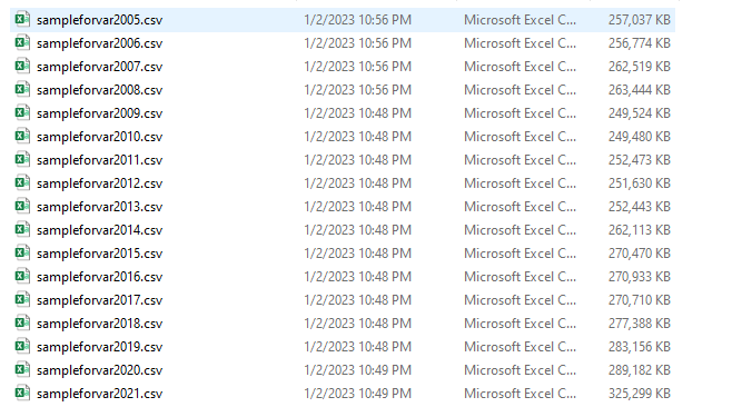
The output of this step is as follows. The raw data for each year is stored in csv file named as sampleforvar + year.

Figure 1: Sample List

Clean Data

We have two tasks in this step.

1. generate the 3 variables rm, x, and r for VAR estimation
2. set time series, which is the prerequisite for using the svar command

Following Brogaard et al. (2022, RFS), the 3 variables for VAR estimation is constructed as follows.

1. I use Equal-Weighted Return (ewretd in CRSP) in basis points as market return rm
2. I use the daily Holding Period Return (ret in CRSP) in basis points as stock return r
3. I use the daily signed dollar volume in $ thousands as stock order flow x
   • The daily signed dollar volume is defined as the product of daily stock price (prc in CRSP), trading volume (vol in CRSP), and the sign of the stocks’ daily return

To mitigate the impacts of outliers, I winsorized all the above variables at the 5% and 95% levels.

I set the index of trading days within a given stock-year to tag the time series.

The Stata codes are as follows. Note that I use the cusip and year as identifiers. For the convenience of looping over stocks, I generate a unique number cusipcode for each stock.

The output in this step is the yearly dataset named as sampledata +year that is ready for the implementation of the VAR estimation in stock-year level.

* import data
cd C:\Users\xu-m\Documents\testVAR\rawdata2005-2021sas

cap program drop cleanforbrogaard
cap program define cleanforbrogaard
	import delimited "sampleforvar`1'.csv",clear
	destring ret, force replace
	drop if ret==.|prc<0|vol<0
	g r = ret*10000
	g prcsign = cond(ret>0,1,-1)
	g x=vol*prc*prcsign/1000
	g rm = ewretd*10000
	
	winsor2 rm x r, cuts(5 95) replace
	
	encode cusip, g(cusipcode)
	sort cusipcode date
	by cusipcode: g index=_n
	xtset cusipcode index
	
	g year = floor(date[1]/10000)
	
	keep cusip cusipcode year index rm x r
	save sampledata`1',replace
end

forvalues j = 2005/2021{
			cleanforbrogaard `j'
}

Extract Estimation Unit and Set Global Variables

As the VAR estimation is implemented in stock-year level, we need firstly extract the sample for each stock and year with the identifiers cusip and year. All the subsequent manipulations are functioning in the single stock-year dataset as follows.

      +----------------------------------------------------------------------+
     |    cusip         r           x          rm   cusipc~e   index   year |
     |----------------------------------------------------------------------|
  1. | 00032Q10    266.24    637.6158        54.7          1       1   2020 |
  2. | 00032Q10     -1.56   -121.6986      -30.57          1       2   2020 |
  3. | 00032Q10    123.44    190.1839       45.48          1       3   2020 |
  4. | 00032Q10    233.06    243.7433        -.41          1       4   2020 |
  5. | 00032Q10   -599.08    -1396.12    9.139999          1       5   2020 |
     |----------------------------------------------------------------------|
  6. | 00032Q10    251.22    234.7973       29.41          1       6   2020 |
  7. | 00032Q10   -245.06   -288.1359      -12.47          1       7   2020 |
  8. | 00032Q10   -178.28   -149.2384       46.14          1       8   2020 |
  9. | 00032Q10     -16.5    -76.8955        29.2          1       9   2020 |
 10. | 00032Q10    201.65    135.6328       31.06          1      10   2020 |
     |----------------------------------------------------------------------|
 ...
     |----------------------------------------------------------------------|
246. | 00032Q10       400    4548.106      -18.55          1     246   2020 |
247. | 00032Q10    -96.15   -1940.581       38.66          1     247   2020 |
248. | 00032Q10    291.26    4240.543      108.42          1     248   2020 |
249. | 00032Q10    -94.34   -937.4673       -2.77          1     249   2020 |
250. | 00032Q10   -285.71   -2000.298        13.5          1     250   2020 |
     |----------------------------------------------------------------------|
251. | 00032Q10   -588.24   -2000.485      -84.83          1     251   2020 |
252. | 00032Q10     312.5    1369.296      101.55          1     252   2020 |
253. | 00032Q10   -101.01    -862.252      -10.58          1     253   2020 |
     +----------------------------------------------------------------------+

In this step, I also set two global variables that will be repeatedly used in the subsequent procedures.

1. the variable names in the VAR system names
2. the number of observations in the dataset unit rownum

The codes for this step are as follows.

* load dataset unit
use sampledata2020,replace
qui keep if cusipcode == 1
list, nolabel
* set global variables
global names "rm x r"
global rownum = _N

Implement Brogaard Decomposition

For now, we’ve collected all the necessary variables, and get the data ready for Brogaard decomposition. Before we actually start to estimate, I would like to provide a big picture for implementing the Brogaard decomposition in a single stock-year dataset.

The tasks we’re going to resolve are as follows.

1. Estimate the reduced-form VAR in Equation (1), saving the residuals $e$ and variance/covariance matrix of residuals ${\Sigma }_e$

2. Estimate matrix $B$, which specifies the contemporaneous effects among variables in the VAR system

3. Estimate the structural shocks ${ϵ}_t$ and their variance-covariance matrix ${\Sigma }_{ϵ}$

4. Estimate the 15-step cumulative structural IRFs ${\theta }_{rm}$, ${\theta }_x$, ${\theta }_r$, which represent the (permanent) cumulative return responses to unit shocks of the corresponding structural-model innovations

5. Combine the estimated variances of the structural innovations from step 3 with the long-run responses from step 4 to get the variance components and variance shares of each information source using the following formula.
   $$\begin{array}{rl}\text{ MktInfo }& ={\theta }_{r_m}^2{\sigma }_{{\epsilon }_{r_m}}^2\\ \text{ PrivateInfo }& ={\theta }_x^2{\sigma }_{{\epsilon }_x}^2\\ \text{ PublicInfo }& ={\theta }_r^2{\sigma }_{{\epsilon }_r}^2.\end{array}$$

6. Estimate the contemporaneous noise term with the following Equation
   $${\Delta }_s=r_t-a_0-{\theta }_{rm}{ϵ}_{rm,t}-{\theta }_x{ϵ}_{x,t}-{\theta }_r{ϵ}_{r,t}$$
   As we’re only interested in the variance of ${\Delta }_s$, which is by construct the variance from noise, we can ignore the constant term $a_0$ and use the variance of KaTeX parse error: Undefined control sequence: \* at position 10: \Delta_s^\̲*̲ to represent the noise variance instead, where
   KaTeX parse error: Undefined control sequence: \* at position 48: …)=Var(\Delta_s^\̲*̲)\\ \Delta_s^\*…

7. Get variance shares by normalizing these variance components
   $$\begin{array}{rl}\text{ MktInfoShare }& ={\theta }_{r_m}^2{\sigma }_{{\epsilon }_{r_m}}^2/({\sigma }_w^2+{\sigma }_r^2)\\ \text{ PrivateInfoShare }& ={\theta }_x^2{\sigma }_{{\epsilon }_x}^2/({\sigma }_w^2+{\sigma }_r^2)\\ \text{ PublicInfoShare }& ={\theta }_r^2{\sigma }_{{\epsilon }_r}^2/({\sigma }_w^2+{\sigma }_r^2)\\ \text{ NoiseShare }& ={\sigma }_s^2/({\sigma }_w^2+{\sigma }_r^2).\end{array}$$

Estimate VAR Coefficients, Matrix $B$, ${ϵ}_t$, ${\Sigma }_e$, and ${\Sigma }_{ϵ}$

I set the lag order as 5 to keep consistent with Broggard et al. (2022, RFS) and then I use svar model to estimate the VAR model, with imposing a Cholesky type restriction to contemporaneous matrix $B$ as mentioned in the paper.

The readers can see details about the matrix $B$ in Dig into Estimation of VAR Coefficients, IRFs, and Variance Decomposition in Stata and see why svar command can directly estimate it in Estimations of VAR, IRFs, and Variance Decomposition in Stata.

The codes for estimating the reduced-form model are as follows.

* estimate B and coefficients of VAR
matrix A1 = (1,0,0 \ .,1,0 \ .,.,1)
matrix B1 = (.,0,0 \ 0,.,0 \ 0,0,.)
qui svar rm x r, lags(1/5) aeq(A1) beq(B1)

The svar command stores the matrix $B$ as e(A), the coefficient matrix as e(b_var) and the variance/covariance matrix of residuals ${\Sigma }_e$ as e(Sigma). So I didn’t estimate them once more but just take them directly from the results of svar estimation.

* store parameter matrix
mat B = e(A)
mat coef = e(b_var)
mat sigma_hat = e(Sigma)

I adjust the freedom of variance/covariance matrix of residuals generated from svar command sigma_hat from $n$ to $n-1$ and name the adjusted variance/covariance matrix as sigma_e. It shouldn’t make much difference if the readers ignore this step.

By definition,
$${ϵ}_t=B{e}_t$$
That also implies
$${\Sigma }_{ϵ}=B{\Sigma }_{e}B$$
With above formulas, we can calculate the structural shocks ${ϵ}_t$ and their variance/covariance matrix ${\Sigma }_{ϵ}$ as follows. I stored the structural shocks in a matrix named epsilons and the variance/covariance matrix of structural shocks in a matrix named sigma_epsilon.

** get residuals e_t
foreach var of varlist rm x r{
	qui cap predict e_`var', resi equation(`var')
}

** get epsilons
mkmat e_rm e_x e_r, matrix(resi)
mat epsilons = (B*resi')'

* get variance-covariance matrix of residuals and epsilons
mat sigma_e = sigma_hat*_N/(_N-1)
mat sigma_epsilon = B*sigma_e*B'

Estimate 15-step cumulative structural IRFs ${\theta }_{rm}$, ${\theta }_x$, and ${\theta }_r$

While the svar command can easily produce the results for IRFs, Orthogonalized IRFs, and Orthogonalized Structural IRFs automatically, what we need are the un-orthogonalized Structural IRFs.

Procedures for estimating $\theta$

These un-orthogonalized Structural IRFs can be quickly and conveniently calculated via the following procedures (please see more details in Dig into Estimation of VAR Coefficients, IRFs, and Variance Decomposition in Stata).

1. calculate the IRFs ${\Phi }_i(i=1,2,\mathrm{3...},15)$ following the following formula, where $k$ is the number of variables in the VAR system. $A_j$ is the $j$-lag coefficient matrix for the reduced-form VAR

$$\begin{gathered} {\Phi }_0=I_k \\ {\Phi }_i={\Sigma }_{j=1}^i{\Phi }_{i-j}{A}_j\text{\hspace{1em}(2)} \end{gathered}$$

2. post-multiply IRF ${\Phi }_i$ with $B^{-1}$ to get (un-orthogonalized) structural IRFs ${\Lambda }_i$ for each forward-looking step $i=1,2,3,..,15$
   $${\Lambda }_i={\Phi }_i{B}^{-1}\text{\hspace{1em}(3)}$$

3. Sum all the 15-step (un-orthogonalized) structural IRFs ${\Lambda }_i$ to obtain the cumulative structural IRFs.

4. As we are only interested in the 15-step cumulative structural IRFs functioning on the stock returns, which are specified in the third equation in the VAR system, the ${\theta }_{rm}$, ${\theta }_x$, and ${\theta }_r$ lie on the third row of the 15-step cumulative structural IRF matrix.

Obtain coefficient matrix $A_j(j=1,2,...,5)$

To implement the above procedures, the first thing we need to get are the reduced-form coefficient matrix $A_j(j=1,2,...,5)$. As we have obtained all the reduce-form coefficients with svar command and stored them in a matrix coef in the last step, we don’t have to compute them again but just need to reshape the matrix coef into the shape we need.

The coefficient matrix we currently have coef is a $1\times 48$ matrix. I first reshape it to a $3\times 16$ matrix named newcoef, where each row contains the coefficients for one equation in the VAR system. Within each row, the coefficients are ordered with fixed rules: the coefficients for the first variable rm with 1 to 5 lags, the coefficients for the second variable x with 1 to 5 lags, the coefficients for the third variable x with 1 to 5 lags, and the constant for the corresponding equation. That implies, the coefficients for the same lag can always be found every 5 columns.

With the above observations, I generated matrix $A_1$ to $A_5$ with the following codes.

* reshape coeficient matrix
cap mat drop newcoef
forvalues i = 1/3{
	mat temp= coef[1..1, 1+16*(`i'-1)..16*`i']
	mat newcoef = nullmat(newcoef) \ temp
}

* generate a1 to a5
forvalues i = 1/5{
	mat A`i' = (newcoef[1..3,`i'], newcoef[1..3,`i'+5], newcoef[1..3,`i'+10])
	mat rownames A`i' = $names
	mat colnames A`i' = $names
	}

I list the 3-lag coefficient matrix $A_3$ as an example to show the desired format of coefficient matrix $A_1$ to $A_5$. For the $ij$-th element of the matrix $A_j$, it represents the impact of one-unit reduced-form shock $e_{jt}$ on the Equation with variable $i$ as dependent variable.

. mat list A3

A3[3,3]

            inflation      unrate         ffr
inflation  -.06574644   .00181085  -.00500138
   unrate   1.4581185   .04263687   -1.835178
      ffr  -.01217184  -.00032878  -.06017122

Calculate IRFs and cumulative un-orthogonalized Structural IRFs

To this stage, we’ve made it clear about the formulas of calculating the IRFs and un-orthogonalized Structural IRFs (please see Equation (2) and (3)) and obtained all the necessary ingredients (coefficient matrix $A_i$ and matrix $B$) for the calculations.

The codes for calculating IRFs and cumulative un-orthogonalized Structural IRFs are as follows. I summed up all the un-orthogonalized Structural IRF matrix step by step to get the 15-step cumulative un-orthogonalized Structural IRFs and name it as csirf.

* calculate IRFs and cumulative un-orthogonalized Structural IRFs
mat irf0 = I(3)
mat sirf0 = irf0*inv(B)
mat csirf = sirf0
forvalues i=1/15{
	mat irf`i' = J(3,3,0)
    forvalues j = 1/5{
    if `i' >= `j'{
        local temp = `i'-`j'
        mat temp2 = irf`temp'*A`j'
        mat irf`i' = irf`i'+ temp2
    }
	}
    mat sirf`i' = irf`i'*inv(B)
    mat csirf = csirf + sirf`i'
}
mat rownames csirf = $names

Extract $\theta$

The 15-step cumulative un-orthogonalized Structural IRF matrix csirf is as follows. The $ij$-th element of this matrix represents the permanent (cumulative) impact of one-unit structural shock ${ϵ}_{j,t}$ on the $i$-th Equation in the VAR system.

. mat list csirf

csirf[3,3]
            rm           x           r
rm   1.0590505   .00356754   .00036924
 x   11.662946   .84352094  -1.0125034
 r   .94265444   .01400394   .76133195

By definition, the elements in the 3rd row of the matrix csirf are ${\theta }_{rm}$, ${\theta }_x$, and ${\theta }_r$ respectively.

Thus, we can extract thetas from the matrix csirf and save the thetas into a new matrix named theta.

* extract thetas
mat theta = csirf[3..3, 1..3]

Calculate noise term

As we’ve discussed in the road map, the noise variance is given by the following formula.
KaTeX parse error: Undefined control sequence: \* at position 48: …)=Var(\Delta_s^\̲*̲)\\ \Delta_s^\*…
Intuitively, we need to first calculate ${\Delta }_s^{\ast }$ by substracting the combinations of structural shocks ${ϵ}_t$ and the permanent impact of structural shocks on stock returns $\theta$ from the contemporaneous stock return $r_t$.

As we’ve saved the structural shocks ${ϵ}_t$ in a matrix named epsilons and the permanent impact of structural shocks on stock returns $\theta$ in a matrix named theta, the contemporaneous noise term ${\Delta }_s^{\ast }$ can be calculated with the following codes, where I save the noise term into a matrix named delta_s.

To more conveniently produce the variance of the noise term, I saved the noise term matrix delta_s into a new column named delta_s in the dataset.

* calculate noise
mkmat r, matrix(r)
mat delta_s = r - (theta*epsilons')'
mat colnames delta_s = "delta_s"
svmat delta_s, names(col)

Calculate the variance from each component

Till now, we’ve collected all the ingredients needed to compute the variance contribution of all the four components defined by the Brogaard et al. (2022, RFS).

Firstly, we calculate the variance contribution from three-types of information with the following formula.
$$\begin{array}{rl}\text{ MktInfo }& ={\theta }_{r_m}^2{\sigma }_{{\epsilon }_{r_m}}^2\\ \text{ PrivateInfo }& ={\theta }_x^2{\sigma }_{{\epsilon }_x}^2\\ \text{ PublicInfo }& ={\theta }_r^2{\sigma }_{{\epsilon }_r}^2.\end{array}$$
As we’ve saved the thetas in a matrix theta and the variance/covariance matrix of structural shocks ${ϵ}_t$ into a matrix sigma_epsilon, we can calculate the information-based variances as follows.

** calculate information part variance
mat var_epsilon = vecdiag(sigma_epsilon)
mat brogaard = J(1,3,0)
forvalues i = 1/3{
	mat brogaard[1,`i']=theta[1, `i']^2*var_epsilon[1, `i']
}
mat brogaard = (brogaard\theta\var_epsilon)
mat rownames brogaard = varpart theta var_epsilon
mat colnames brogaard = $names

Note that I put all the variance components along with the related parameters $\theta$ and ${\sigma }_{ϵ}$ into a new matrix named brogaard. This matrix looks like as follows.

. mat list brogaard

brogaard[3,3]
                    rm          x          r
    varpart    17851.6  7821.7685  56649.107
      theta  .94265444  .01400394  .76133195
var_epsilon  20089.638   39884558   97733.84

Secondly, I calculate the variance contribution from noise, which is proxied by the variance of ${\Delta }_s^{\ast }$ we’ve calculated above. Of course, I add the noise variance into the result matrix brogaard.

** calculate noise part variance
mat brogaard = (brogaard, J(3,1,0))' 
qui sum delta_s
mat brogaard[4,1] = r(sd)^2
mat rownames brogaard = $names "s"

After this step, we’ve figured out the variance contribution from each component defined by the Brogaard paper and saved them into the result matrix brogaard.

The final result matrix brogaard is as follows.

. mat list brogaard

brogaard[4,3]
        varpart        theta  var_epsilon
rm      17851.6    .94265444    20089.638
 x    7821.7685    .01400394     39884558
 r    56649.107    .76133195     97733.84
 s    20275.294            0            0

Calculate variance contribution

To more conveniently calculate the variance contribution, I saved the result matrix brogaard into the dataset. I follow the following formula to calculate the variance contribution of each component and save the percentages into a new variable named varpct.
$$\begin{array}{rl}\text{ MktInfoShare }& ={\theta }_{r_m}^2{\sigma }_{{\epsilon }_{r_m}}^2/({\sigma }_w^2+{\sigma }_r^2)\\ \text{ PrivateInfoShare }& ={\theta }_x^2{\sigma }_{{\epsilon }_x}^2/({\sigma }_w^2+{\sigma }_r^2)\\ \text{ PublicInfoShare }& ={\theta }_r^2{\sigma }_{{\epsilon }_r}^2/({\sigma }_w^2+{\sigma }_r^2)\\ \text{ NoiseShare }& ={\sigma }_s^2/({\sigma }_w^2+{\sigma }_r^2).\end{array}$$

keep cusip year
qui keep in 1/4
qui svmat brogaard, names(col)
qui g rownames = ""
local index = 1
foreach name in $names "s"{
	qui replace rownames = "`name'" if _n == `index'
	local index = `index' + 1
}
egen fullvar = sum(varpart)
qui g varpct = varpart/fullvar*100

Pack codes

Remember the Broggard decomposition is implemented in stock-year level. That means we need to loop over the above codes over the daily observations of each stock in each year. That requires an efficient packing of the codes.

There are two issues worth noted in the packing procedures.

1. I require there are at least 50 observations for the estimation of the VAR model
   • otherwise, the VAR estimation doesn’t converge or lacks vaidility with too few freedoms
2. I require the estimation of VAR model converges
   • otherwise, it’s not possible to get converged residuals, which are the prerequisite for the subsequent calculations

cap program drop loopb
cap program define loopb
	use sampledata`2',replace
	qui keep if cusipcode == `1'
	
	if _N >= 50{
	* set global variables
	global names "rm x r"
	global rownum = _N

	* estimate B and coefficients of VAR
	matrix A1 = (1,0,0 \ .,1,0 \ .,.,1)
	matrix B1 = (.,0,0 \ 0,.,0 \ 0,0,.)
	qui svar rm x r, lags(1/5) aeq(A1) beq(B1)
	mat B = e(A)
	mat coef = e(b_var)
	mat sigma_hat = e(Sigma)

	* get coefficient matrix of var a1-a5
	* reshape coeficient matrix
	cap mat drop newcoef
	forvalues i = 1/3{
		mat temp= coef[1..1, 1+16*(`i'-1)..16*`i']
		mat newcoef = nullmat(newcoef) \ temp
	}

	* generate a1 to a5
	forvalues i = 1/5{
		mat A`i' = (newcoef[1..3,`i'], newcoef[1..3,`i'+5], newcoef[1..3,`i'+10])
		mat rownames A`i' = $names
		mat colnames A`i' = $names
		}

	* get 15-step coefficients of VMA (irf), structual irf (sirf), and cumulative sirf
	mat irf0 = I(3)
	mat sirf0 = irf0*inv(B)
	mat csirf = sirf0
	forvalues i=1/15{
		mat irf`i' = J(3,3,0)
		forvalues j = 1/5{
		if `i' >= `j'{
		local temp = `i'-`j'
		mat temp2 = irf`temp'*A`j'
		mat irf`i' = irf`i'+ temp2
	}
	}
		mat sirf`i' = irf`i'*inv(B)
		mat csirf = csirf + sirf`i'
	}

	* extract thetas
	mat theta = csirf[3..3, 1..3]

	* get reisduals, epsilons, and their variance-covariance matrix
	** get residuals
	foreach var of varlist rm x r{
		qui cap predict e_`var', resi equation(`var')
	}
	
	capture confirm variable e_rm
	if (_rc == 0){
			** get epsilons
		mkmat e_rm e_x e_r, matrix(resi)
		mat epsilons = (B*resi')'

		** get variance-covariance matrix of residuals and epsilons
		mat sigma_e = sigma_hat*_N/(_N-1)
		mat sigma_epsilon = B*sigma_e*B'

		* calculate noise
		mkmat r, matrix(r)
		mat delta_s = r - (theta*epsilons')'
		mat colnames delta_s = "delta_s"
		svmat delta_s, names(col)

		* calculate variance decomposition of each part
		** calculate information part variance
		mat var_epsilon = vecdiag(sigma_epsilon)
		mat brogaard = J(1,3,0)
		forvalues i = 1/3{
			mat brogaard[1,`i']=theta[1, `i']^2*var_epsilon[1, `i']
		}
		mat brogaard = (brogaard\theta\var_epsilon)
		mat rownames brogaard = varpart theta var_epsilon

		** calculate noise part variance
		mat brogaard = (brogaard, J(3,1,0))' 
		qui sum delta_s
		mat brogaard[4,1] = r(sd)^2
		mat rownames brogaard = $names "s"
		*mat list brogaard

		** save the variance decomposition results 
		keep cusip year
		qui keep in 1/4
		qui svmat brogaard, names(col)
		qui g rownames = ""
		local index = 1
		foreach name in $names "s"{
			qui replace rownames = "`name'" if _n == `index'
			local index = `index' + 1
		}
		egen fullvar = sum(varpart)
		qui g varpct = varpart/fullvar*100

		* save final results
		local savename = "C:\Users\xu-m\Documents\testVAR\resvardecompose\brogaard_'$cusip'_$year.dta"
		qui save "`savename'", replace
	}
	}
end 

Loop over sample

I run the packed code over stocks in each year and collected all the results for different years together. Then I reshaped the dataset into panel data. The codes are as follows.

cd C:\Users\xu-m\Documents\testVAR\resvardecompose

* collect results for each year
cap program drop collectbroggardbyyear
cap program define collectbroggardbyyear
	clear
	set obs 0
	save brogaard`1', replace emptyok

	local ff : dir . files "*_`1'.dta"
	local yearnum : word count "`ff'"
	local index = 1
	foreach f of local ff {
		append using "`f'"
		di "`index' of `yearnum' in year `1'"
		local index = `index' + 1
		}
	save brogaard`1', replace 
end

* collect all years
clear 
set obs 0
save ../brogaard, replace emptyok
forvalues year = 2005/2021{
	collectbroggardbyyear `year'

	use ../brogaard, replace
	append using brogaard`year'
	save ../brogaard, replace 
}

* reshape into panel data
cd ../

use brogaard, replace
rename fullvar_r sdr
replace rownames = "_"+rownames
reshape wide varpart theta var_epsilon fullvar varpct sdr, i(cusip year) j(rownames) string
rename varpct_rm mktinfo
rename varpct_x privteinfo
rename varpct_r publicinfo
rename varpct_s noise
keep cusip year *info noise
save panelbrogaard, replace

The final outcome is as follows.

. list in 1/20

     +-------------------------------------------------------------+
     |    cusip   year   public~o    mktinfo      noise   privte~o |
     |-------------------------------------------------------------|
  1. | 00030710   2014   .4612017   17.60379   58.85497   23.08004 |
  2. | 00030710   2015   43.65164   10.60914   12.57214   33.16709 |
  3. | 00030710   2016   41.93059   13.32436   6.182855    38.5622 |
  4. | 00030710   2017   54.59381   1.191425   14.96389   29.25087 |
  5. | 00030710   2018     43.838   25.09339   8.907529   22.16108 |
     |-------------------------------------------------------------|
  6. | 00030710   2019   30.02275   25.98764   12.31215   31.67746 |
  7. | 00032Q10   2018   18.90079   23.99627   36.99344   20.10949 |
  8. | 00032Q10   2019   59.49644   5.478648   11.91035   23.11457 |
  9. | 00032Q10   2020   55.21476    17.3996   19.76192   7.623722 |
 10. | 00032Q10   2021   51.75403   25.38084   12.44535   10.41978 |
     |-------------------------------------------------------------|
 11. | 00036020   2005   40.70956   7.924543   26.06547   25.30043 |
 12. | 00036020   2006   38.53111   21.68062   6.496971   33.29131 |
 13. | 00036020   2007   32.78075   4.495751   27.55989    35.1636 |
 14. | 00036020   2008   21.36486   47.52046   16.44107    14.6736 |
 15. | 00036020   2009   34.37528   31.25706   17.96114   16.40653 |
     |-------------------------------------------------------------|
 16. | 00036020   2010   39.55574   34.02036   8.709065   17.71484 |
 17. | 00036020   2011   21.50586   17.19429   46.27998   15.01987 |
 18. | 00036020   2012    52.9045   11.12552   11.89774   24.07223 |
 19. | 00036020   2013   12.02968   14.62235   16.48395   56.86403 |
 20. | 00036020   2014   31.94392   42.19098   8.426245   17.43885 |
     +-------------------------------------------------------------

Conclusion

In this blog, I replicated the stock volatility decomposition method introduced by Brogaard et al. (2022, RFS). Given the potential of this information-based decomposition method as I’ve discussed in Theory for the information-based decomposition of stock price, I hope this blog can help the readers make use of this method to empower their own research.