Field II 超声声场仿真(1): 发射声场(原理&代码)

系列一：利用Field II仿真计算发射声场强度

0. 基本参数定义

c = 1540;                   % Speed of sound
f0 = 2.5e6;                 % Transducer center frequency [Hz]
fs = 100e6;                 % Sampling frequency [Hz]
lambda = c/f0;              % Wavelength
element_height = 13/1000;   % Height of element [m] (elevation direction)
element_width = 18.5/1000;  % Element width [m] (azimuth direction)
kerf = 0;
focus = [0 0 60]/1000;      % Fixed emitter focal point [m] (irrelevant for single element transducer)
N_elements = 1;             % Number of physical elements in array
N_sub_x = 1;                % Element sub division in x-direction
N_sub_y = 1;                % Element subdivision in y-direction

1. 定义发射孔径

在Filed II中使用xdc_命令设置换能器的基本参数，xdc_linear_array命令创建一个线阵换能器。

emit_aperture = xdc_linear_array (N_elements, element_width, element_height, kerf, N_sub_x, N_sub_y, focus);

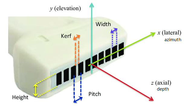
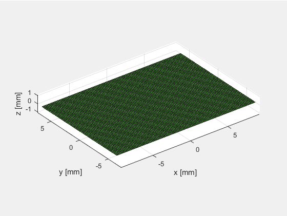
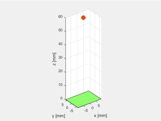
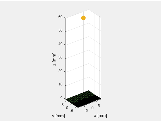
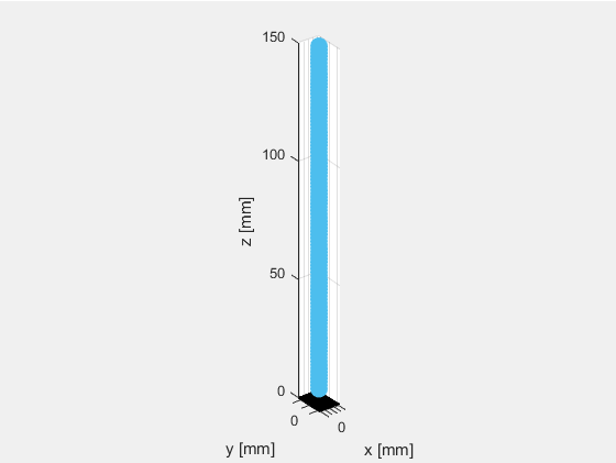
#####1.1 单阵元换能器

定义单阵元换能器，阵元个数为1，x和y方向上的子阵个数也设置为1：N_elements = 1, N_sub_x=1; N_sub_y=1.
绘制换能器，结果如下图所示。

可以看出当阵元数等于1时(N_elements=1)，阵元在x轴方向上的长度等于element_width，在y轴方向上的宽度等于element_height。而N_sub_x和N_sub_y只是进行进一步的子阵划分，并不影响仿真计算的结果。

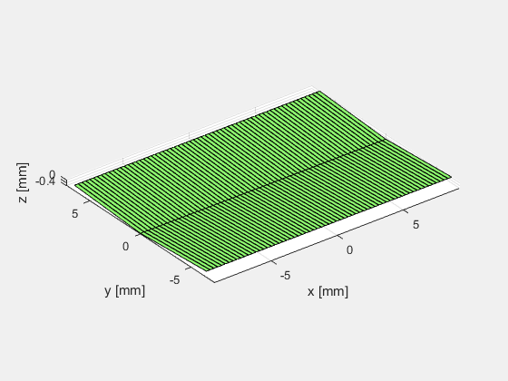
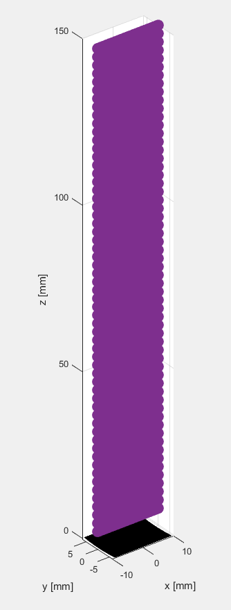
#####1.2 换能器阵列

使用xdc_focus_array指令创建聚焦换能器阵列，如下图所示

element_height = 13/1000;   % Height of element [m] (elevation direction)
pitch = 0.290/1000;         % Distance between element centers
kerf = 0.025/1000;          % Width of fill material between the ceramic elements
element_width = pitch-kerf; % Element width [m] (azimuth direction)
Rfocus = 60/1000;           % Elevation lens focus (or radius of curvature, ROC) 
focus = [0 0 60]/1000;      % Fixed emitter focal point [m] (irrelevant for single element transducer)
N_elements = 64;            % Number of physical elements in array
N_sub_x = 1;                % Element sub division in x-direction
N_sub_y = 2;                % Element subdivision in y-direction

emit_aperture = xdc_focused_array (N_elements, element_width, element_height, kerf, Rfocus, N_sub_x, N_sub_y, focus);

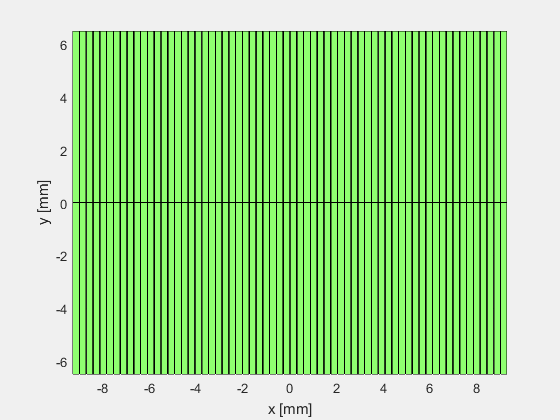
其中，Rfocus定义了换能器的曲率半径。

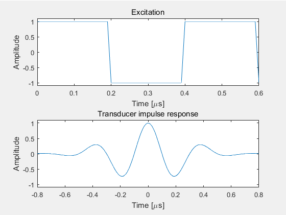
2. 设置换能器的激励和脉冲响应

定义好发射孔径之后，使用xdc_excitation()函数设置发射孔径的激励脉冲Excitation，此处设置激励脉冲的中心频率为2.5MHz，脉冲长度为1.5个周期。

ex_periods = 1.5;
t_ex=(0:1/fs:ex_periods/f0);
excitation=square(2*pi*f0*t_ex);
xdc_excitation (emit_aperture, excitation);

之后，使用xdc_impulse()函数设置换能器发射孔径的脉冲响应Transducer impulse response.

t_ir = -2/f0:1/fs:2/f0;
Bw = 0.6;    %带宽设为0.6
impulse_response=gauspuls(t_ir,f0,Bw);
set_sampling(fs);
xdc_impulse (emit_aperture, impulse_response);

3. 计算发射声场强度

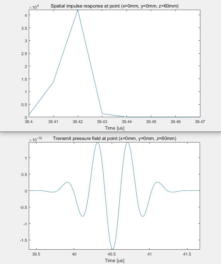
#####3.1 一个点处的声场强度

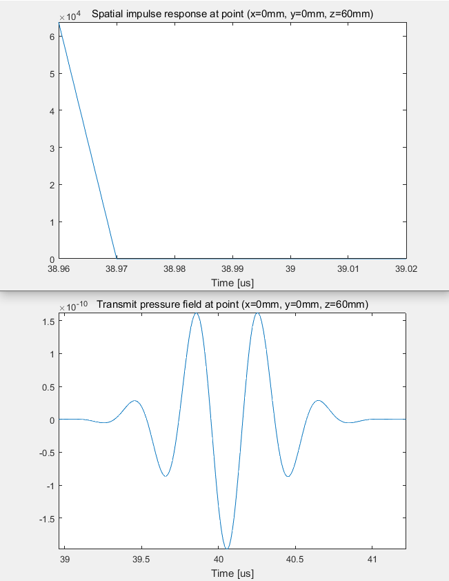
比如，选择(0, 0, 60)mm处为测量点。

使用calc_h()函数计算该点处的空间脉冲响应Spatial impulse response.

使用calc_hp()函数计算该点处的声场强度Transmit pressure.

(1) 单阵元测量结果

(2) 聚焦换能器阵列测量结果

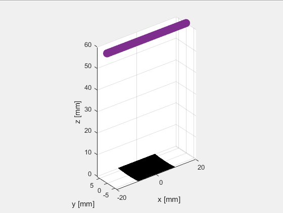
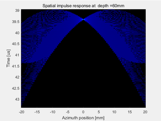
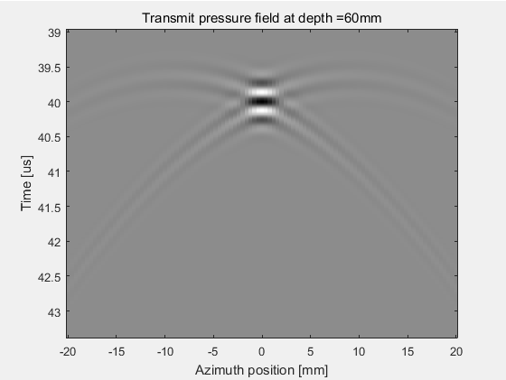
#####3.2 一条线上的声场强度

(1) 横向计算结果

若干点可以组成一条线，在(-20,0,60)mm到(20,0,60)mm处选择101个测量点形成一条线，计算聚焦换能器阵列在60mm深度处的空间脉冲响应和声场强度。

(2) 径向计算结果：计算声轴上声压分布

在(0,0,5)mm到(0,0,150)mm处选择101个测量点形成一条测量线

改变焦点位置

Rfocus = 60/1000;           % Elevation lens focus (or radius of curvature, ROC) 
focus = [0 0 30]/1000;      % Fixed emitter focal point [m] (irrelevant for single element transducer)

改变换能器阵元数，从64减少至32

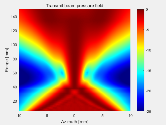
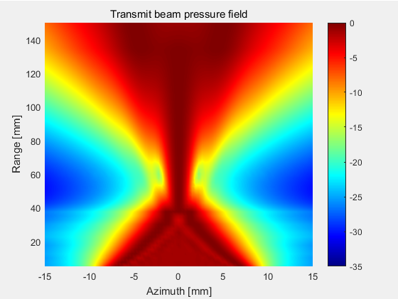
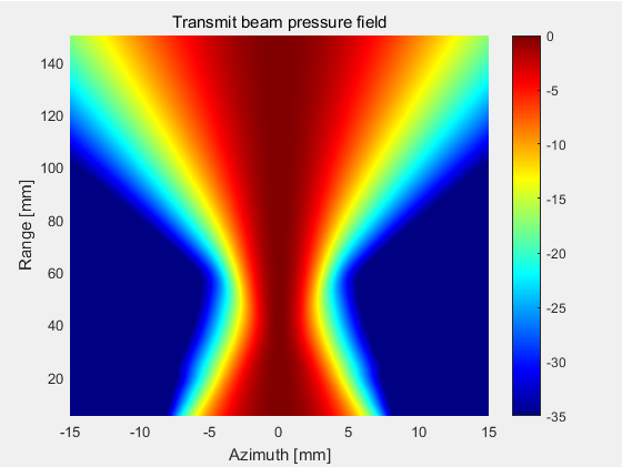
3.3 一个平面的声场强度(xz平面)

选择81x59个测量点，计算xz切面方向上的声场强度，其中x的变化范围为-15mm至15mm，z的变化范围为5mm至150mm。

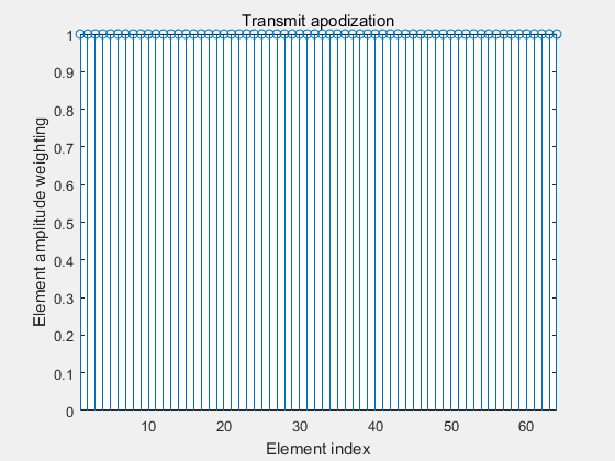
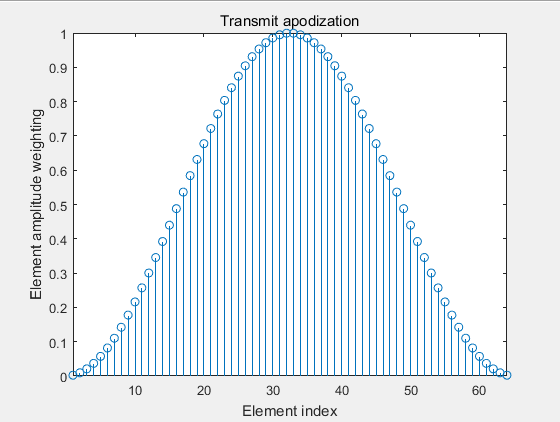
4. 增加变迹函数

4.1 boxcar变迹函数

4.2 Hanning变迹函数

代码请加QQ：2971319104