你需要知道的一些深度学习的论文(卷积神经网络-初学者指南 (Part 3))

原文:传送门

本文介绍你需要知道的有关深度学习的论文。

这里写图片描述

卷积神经网络-初学者指南 (Part 1)
卷积神经网络-初学者指南 (Part 2)

简介

本文,我们总结了计算机视觉及卷积神经网络领域重要的里程碑。我们将介绍近5年发表的最重要的论文,并讨论它们为什么重要。本文前半部分(从AlexNet到ResNet)介绍网络构架的发展,后半部分介绍子领域中有趣的论文。

AlexNet(2012)

这篇论文的标题为“ImageNet Classification with Deep Convolutional Networks”,该论文至今被引用6184次,被视为该领域最具有影响力的论文之一。Alex Krizhevsky,Ilya Sutskever,和Geoffrey Hinton创造了“large, deep convolutional neural network“并赢得2012 ILSVRC(ImageNet Large-Scale Visual Recognition Challenge)。对于那些不熟悉的人来说,可以将其视作一年一度的计算机视觉奥运会,来自世界各地的参数队伍竞相比较,为分类,定位,检测等任务角逐出最好的计算机视觉模型。2012年,CNN开始被用于图像分类,其Top5的错误率为15.4%,而这之前最好的结果为26.2%,这是一个惊人的进步,几乎震惊了计算机视觉社区。从此,CNNs家喻户晓。
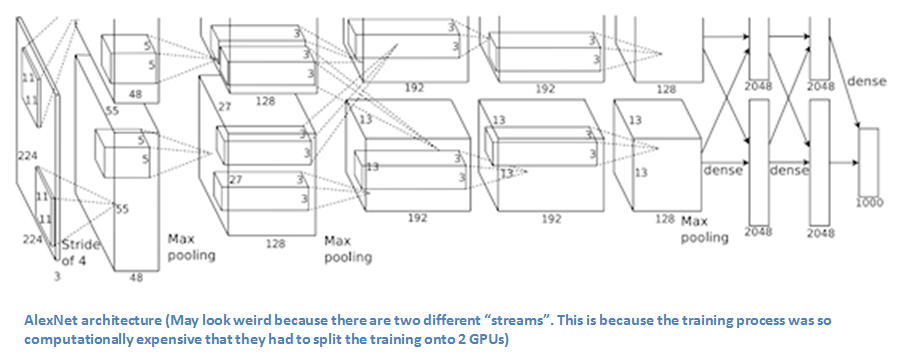
在该论文中,研究小组讨论了AlexNet的网络结构。与现在的模型相比,他们使用了相对简单的布局。该网络由5个卷积层,max-pooling层,dropout层,以及3个全连接层组成。研究小组设计了一千个可能类别。

这里写图片描述

要点

  • 使用ImageNet数据训练网络。ImageNet数据集包含22000+种类别,1500+万张图片。
  • 使用 ReLU作为非线性函数。
  • 使用了数据增强技术,包括图像平移、水平反射和补丁提取(image translations, horizontal reflections, and patch extractions)。
  • 为了避免过拟合而实现了dropout层
  • 使用批量随机梯度下降,并指定了动量和权重衰减的值。
  • 用两块GTX580 GPU训练了5-6天

为什么重要
这是在ImageNet历史第一个表现如此优秀的模型。它所使用的技术,如数据增强,dropout等,至今仍在使用。该论文用在ImageNet比赛中惊人的表现向世人展示了卷积神经网络的优势。

ZF Net(2013)

随着AlexNet的出彩表现,2013年的ILSVRC上CNN模型数量大增。而该年的冠军是由来着华盛顿大学的 Matthew Zeiler 和 Rob Fergus开发的网络模型。这个网络名为ZF Net, 该模型达到了11.2%的错误率。这个网络大部分是对AlexNet进行了微调,并为其提高了性能。这篇论文优秀的另一个原因是作者花了很长时间来解释ConvNets和如何正确可视化过滤器和权重。
在这篇题为“Visualizing and Understanding Convolutional Neural Networks”的论文中,Zeiler和Fergus开始讨论这种因海量数据集的出现和计算能力提高而复兴的神经网络模型。他们还表明研究人员对这些模型内部机制的理解有限,他们说,如果没有这方面的见解,“再好的模型的开发也会变成尝试和犯错”。虽然我们现在比3年前有更好的理解,但这仍然是许多研究人员的问题!本文的主要贡献是稍微修改AlexNet模型的细节并展示一个非常有趣的可视化特征图。

这里写图片描述

要点

  • 除了一小点改动,其结构与AlexNet有非常相似。
  • AlexNet用来1500万张图像去训练,而ZF Net只用了130万张图像。
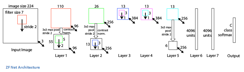
  • AlexNet在第一层用了尺寸为11*11的过滤器,而ZF Net用了尺寸为7*7的过滤器,且减小了步长。这一改动的原因是:在第一层,更小的过滤器可以保存更多的原始图像信息。而11*11的过滤器跳过了很多相关信息,尤其是在第一层。
  • 随着网络的发展,我们可以看到网络中过滤器的数量在增加。
  • 使用ReLU作为激活函数,交叉熵损失作为损失函数,并使用批量随机梯度下降。
  • 使用 1块 GTX 580 GPU训练12天。
  • 开发了一个名为Deconvolutional Network(反卷积网络)的可视化技术,用于研究不同特征激活和输入空间的关系。之所以称它“Deconvenet”(反卷积),是因为它将特征映射回像素空间(与卷积层正好相反)。

DeConvNet
这项技术的基本思路是在CNN训练完成后,你使用deconvnet将每层的特征映射回像素空间。一般,作为前向过程,输入的图像被喂给CNN然后在每一层的计算激活。现在,假设我们要检查下第4层特征的激活。我们会保存这一特征映射的激活,将该层上的其他激活设为0,然后将该特征作为输入喂给deconvnet。deconvnet具有和原始CNN相同的过滤器。输入的特征经过每个层一系列的反池化(unpooling),整流(rectify),和过滤操作直到原始的输入像素空间。
整个过程背后的原因是,我们想研究是什么类型的结构激活了特征。让我们看看第一层和第二层的可视化。

这里写图片描述
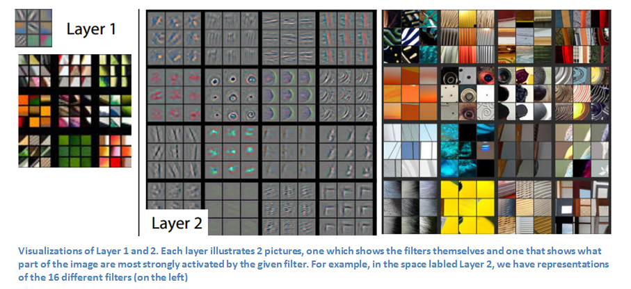
第一层和第二层的可视化。从这两张图片中,很容易看出对于给定的过滤器,哪个部分得到的激活最强

像在Part1讨论的那样,卷积网络的第一层总是一些低层次的特征检测,他们回去检测图片中的边缘和颜色。我们可以在第二层中看到很多的环形特征被检测出来。让我们再看下第3,4,5层的特征。

这里写图片描述

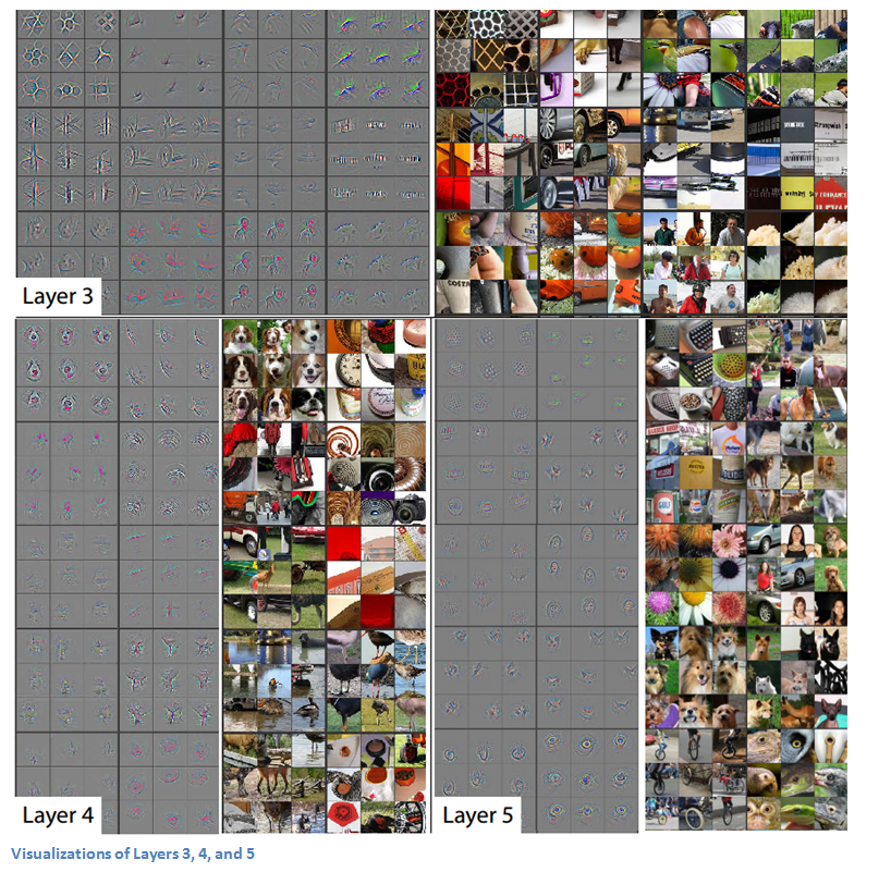
这些层展示了更高层次的特征,比如狗的脸和花。有一点要注意的是,你可能还记得,第一次转换层后,我们通常有一个汇聚层(pooling),下采样的图像(例如,变成一个32x32x3体积为16x16x3卷)。这样做的使得第二层的过滤器可以“看”到更广阔的范围。想知道更详细的信息可以观看Zeiler的报告视频(来自不存在的youtube)。

为什么重要?
ZF Net 不仅是2013年ILSVRC的冠军,还提供了许多提高CNN性能的方法并对CNN如何工作有了一个直观的理解。可视化的方法不仅有助于解释神经网络的内部运作,而且还为网络体系结构的改进提供了方法。迷人的deconv可视化方法和遮挡实验(论文中一个实验)使其成为我最喜欢的一片论文之一。

VGG Net(2014)

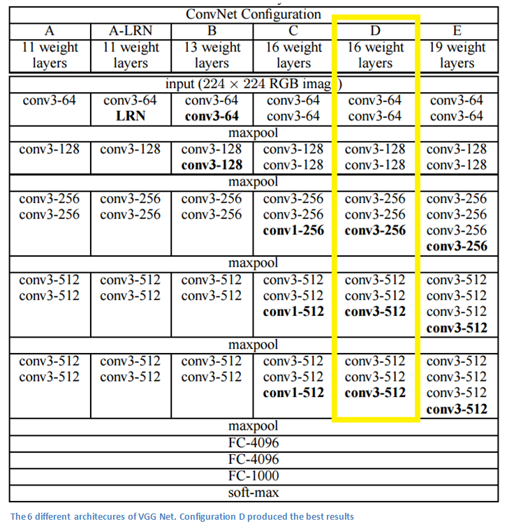
简单的,深的。来自牛津大学的Karen Simonyan 和 Andrew Zisserman 用这一理念创造了这个19层的CNN模型,所有层使用尺寸3*3,步长为1的过滤器,填充为1,并使用了尺寸2*2,步长为2的max-pooling层。最后获得了错误率为7.3%(并不是ILSVRC 2014的冠军)。

这里写图片描述

要点

  • 仅使用3*3的过滤器。与AlexNet和ZF Net在过滤器方面相差较大。根据作者的推理,连续两层3*3的卷积层要比一层5*5的卷积层的感受野更有效率。用较小的过滤器去模拟较大的过滤器会有以下好处:1.减少参数数量。2.两层的卷积层使得我们能加入两层ReLU,加入了更多非线性。

这里借用cs231n中的一张PPT结果例子,帮助理解:
(PS:原文没有,我自己加的,不感兴趣可以跳过)

这里写图片描述


  • 每层的输入都在减少(由于卷积层和pooling层的作用),但由于卷积层增多,网络深度加深。
  • 在图像分类和定位任务中表现很好。作者将定位任务的结构用于回归。(详见论文第10页)
  • 用Caffe训练模型。
  • 采用scale jittering 数据增强技术。
  • 在每个卷积层后面使用ReLU并用批量随机下降训练。
  • 使用4个Nvidia Titan Black GPU 训练2-3周。

为什么重要?
VGG Net是对我的思想影响最大的论文之一,它进一步强化了为了分层表达可视化数据,CNNs需要更深层网络这一观点。Keep it deep. Keep it simple.

GoogLeNet(2015)

你理解了我们刚刚谈及的网络结构中的简单思想了吗?好吧,Google把它拧巴拧巴丢出了窗外并向你扔了一只Inception module。(译者注:Google真是个神奇的公司,在我翻译这篇博文的时候,又发表了一篇名为《One Model To Learn Them All》,再一次刷新了我对深度学习的认识,他们提出了一种适合多种任务的模型。)GoogLeNet是一个22层的CNN,并以Top-5 6.7%的错误率赢得了2014年的ILSVRC 。在我的理解中,这是第一个与传统的使用conv和pooling层顺序搭建方法不一样的CNN结构。论文的作者还强调,这个新的模型注重对内存和资源的使用。(注意:我有时会忘记:将所有层叠加并增加过滤器的数量会加大计算的储存成本,增加过拟合的风险。)

这里写图片描述

这里写图片描述

Inception Module
当我们第一次看到GoogLeNet的结构的时候,我们马上回意识到这并不是所有事情都在按顺序运行,就像先前图中所示的那样。在网络的一些片段中,我们进行了并行操作。

这里写图片描述

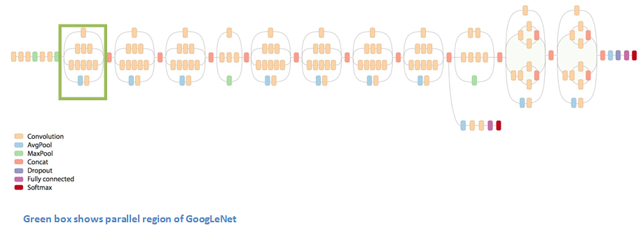
这个结构被称为Inception module。让我们近距离观察下它是由什么构成的。

这里写图片描述

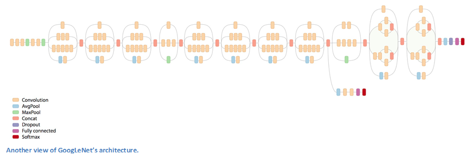
底下绿色的方框是我们的输入,顶上的那个是模型的输出(将这张图片右90度旋转可以让你形象地看到与上面一张显示完整网络的图片有关的模型。)基本上,对于传统卷积神经网络的每一层,你必须从是否pooling操作或卷积(包括过滤器尺寸的选择)操作中作出选择。Inception module允许你并行执行这些操作。事实上,这其实是作者提出的“初级”的想法。

这里写图片描述

那么,为什么不能这样做呢?这回导致太多输出。我们最终会得好一个深度非常大的输出。作者采用的方法是在3*3和5*5卷积层前加上1*1卷积层。这个1*1的卷积层(或者说是Network in network层)提供一个减少维度的方法。比如,你的输入数据块为100*100*60(这并不是图片的维度,可能是网络中的任意层的输入)。使用20个1*1的过滤器可以将让你将输入块减少到100*100*20。这意味着3*3和5*5的卷积层不需要处理太大的数据块。这可以理解为“pooling of features”,因为我们减小了数据块的深度,就像我们通过maxpooling层减少数据的height和width一样。另外需要注意的是,在这些1*1的卷积层后加入ReLU并不对其产生负面影响(更多的信息可以阅读Aaditya Prakash的博文)。推荐该视频(油管视频,需翻墙),对过滤器在最后级联进行有一个直观的理解。
你可能会问自己“这样的结构有什么用呢?”。这个模型包含了network in network layer,中等尺寸的卷积过滤器,大尺寸卷积过滤器及pooling操作。network in network层提取细粒度的细节信息,3*3和5*5过滤器拥有不同范围的感受野也能很好的提取输入中的信息。你还能通过pooling层减少输入空间尺寸而避免过拟合。你可以在这些卷积层后加入ReLU,以提高网络的非线性。基本上,网络可以执行这些不同操作的功能,同时仍能计算周到。论文中还结合稀疏矩阵和稠密矩阵等主题提出了更高层次的推理(阅读论文的第3和第4节。我至今还不是很清楚这其中的意思,如果有人理解,我很愿意与你们在评论中讨论!)

要点

  • 在整个结构中使用了9个Inception module,超过100层!很深的结构…
  • 没有使用全连接层!而是使用average pool,将7*7*1024的数据块变成1*1*1024。
  • 使用了远少于AlexNet的参数。
  • 在测试时,对同一份图片进行裁剪,喂给网络,并使用softmax计算平均值后再给出最终结果。
  • 他们的检测模型利用了R-CNN(这篇论文,稍后会讲)中的概念。
  • 对Inception module进行版本更新。
  • 使用少数高端GPU训练一周。

为什么重要
GoogLeNet 是第一个不使用传统顺序叠加构造方法的模型。提出了Inception module,并展示了该创造性的结构的模型能够提升模型表现并且使网络更有效率的进行计算。这个模型为未来几年内出现的具有惊人结构的模型搭建了平台。

这里写图片描述

Microsoft ResNet(2015)

想象一下将一个卷积神经网络结构的层数翻倍,但可能得到的深度依然没有比2015有微软亚研院提出的ResNet结构深。ResNet是一个新型的拥有152层结构的网络。在层数方面的创造了新纪录的同时,ResNet也将错误率减少到惊人的3.6%并赢得了2015年的ILSVRC。
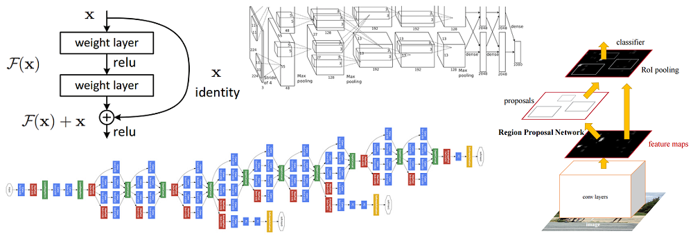
这里写图片描述

Residual Block
Residual Block的思路是将你的输入x进过conv-relu-conv转换后,得到F(x)。然后加上原始的输入x。我们将其称为H(x)=F(x)+x。在传统的神经网络中,我们的H(x)是等于F(x)的。但是在ResNet中我们向F(x)加入x。我们可以下面的模块看成是对原始输入x加上一些“增量”或者做了一些轻微的改变。ResNet的作者认为ResNet的优化比原始的优化要简单。

这里写图片描述

这个残余块可能有效的另一个原因是在反向传播的反向传递过程中,梯度很容易通过图传播,因为存在加法运算,可以分配梯度。

要点

  • “超深”——Yann LeCun
  • 152层…
  • 有趣的是,只有前两层,空间大小从输入的224*224减小的56*56。
  • 作者认为无脑的增加层会提高训练和测试的错误率。
  • 研究小组尝试过1202层的网络,但得到的测试准确率很低,也许是因为是过拟合了。
  • 使用8块GPU训练2-3周。

    为什么重要
    3.6%的错误率。这本身就很有说服力。ResNet是目前最好的卷积神经网络模型,它是residual learning思想的伟大创新。我相信我们已经达到了这样的程度:在彼此的模型上叠加更多的层,已经不会带来实质性的提升。

书的目录 Contents Website viii Acknowledgments ix Notation xiii 1 Introduction 1 1.1 Who Should Read This Book? . . . . . . . . . . . . . . . . . . . . 8 1.2 Historical Trends in Deep Learning . . . . . . . . . . . . . . . . . 12 I Applied Math and Machine Learning Basics 27 2 Linear Algebra 29 2.1 Scalars, Vectors, Matrices and Tensors . . . . . . . . . . . . . . . 29 2.2 Multiplying Matrices and Vectors . . . . . . . . . . . . . . . . . . 32 2.3 Identity and Inverse Matrices . . . . . . . . . . . . . . . . . . . . 34 2.4 Linear Dependence and Span . . . . . . . . . . . . . . . . . . . . 35 2.5 Norms . . . . . . . . . . . . . . . . . . . . . . . . . . . . . . . . . 37 2.6 Special Kinds of Matrices and Vectors . . . . . . . . . . . . . . . 38 2.7 Eigendecomposition . . . . . . . . . . . . . . . . . . . . . . . . . . 40 2.8 Singular Value Decomposition . . . . . . . . . . . . . . . . . . . . 42 2.9 The Moore-Penrose Pseudoinverse . . . . . . . . . . . . . . . . . . 43 2.10 The Trace Operator . . . . . . . . . . . . . . . . . . . . . . . . . 44 2.11 The Determinant . . . . . . . . . . . . . . . . . . . . . . . . . . . 45 2.12 Example: Principal Components Analysis . . . . . . . . . . . . . 45 3 Probability and Information Theory 51 3.1 Why Probability? . . . . . . . . . . . . . . . . . . . . . . . . . . . 52 i CONTENTS 3.2 Random Variables . . . . . . . . . . . . . . . . . . . . . . . . . . 54 3.3 Probability Distributions . . . . . . . . . . . . . . . . . . . . . . . 54 3.4 Marginal Probability . . . . . . . . . . . . . . . . . . . . . . . . . 56 3.5 Conditional Probability . . . . . . . . . . . . . . . . . . . . . . . 57 3.6 The Chain Rule of Conditional Probabilities . . . . . . . . . . . . 57 3.7 Independence and Conditional Independence . . . . . . . . . . . . 58 3.8 Expectation, Variance and Covariance . . . . . . . . . . . . . . . 58 3.9 Common Probability Distributions . . . . . . . . . . . . . . . . . 60 3.10 Useful Properties of Common Functions . . . . . . . . . . . . . . 65 3.11 Bayes’ Rule . . . . . . . . . . . . . . . . . . . . . . . . . . . . . . 68 3.12 Technical Details of Continuous Variables . . . . . . . . . . . . . 69 3.13 Information Theory . . . . . . . . . . . . . . . . . . . . . . . . . . 71 3.14 Structured Probabilistic Models . . . . . . . . . . . . . . . . . . . 73 4 Numerical Computation 78 4.1 Overflow and Underflow . . . . . . . . . . . . . . . . . . . . . . . 78 4.2 Poor Conditioning . . . . . . . . . . . . . . . . . . . . . . . . . . 80 4.3 Gradient-Based Optimization . . . . . . . . . . . . . . . . . . . . 80 4.4 Constrained Optimization . . . . . . . . . . . . . . . . . . . . . . 91 4.5 Example: Linear Least Squares . . . . . . . . . . . . . . . . . . . 94 5 Machine Learning Basics 96 5.1 Learning Algorithms . . . . . . . . . . . . . . . . . . . . . . . . . 97 5.2 Capacity, Overfitting and Underfitting . . . . . . . . . . . . . . . 108 5.3 Hyperparameters and Validation Sets . . . . . . . . . . . . . . . . 118 5.4 Estimators, Bias and Variance . . . . . . . . . . . . . . . . . . . . 120 5.5 Maximum Likelihood Estimation . . . . . . . . . . . . . . . . . . 129 5.6 Bayesian Statistics . . . . . . . . . . . . . . . . . . . . . . . . . . 133 5.7 Supervised Learning Algorithms . . . . . . . . . . . . . . . . . . . 137 5.8 Unsupervised Learning Algorithms . . . . . . . . . . . . . . . . . 142 5.9 Stochastic Gradient Descent . . . . . . . . . . . . . . . . . . . . . 149 5.10 Building a Machine Learning Algorithm . . . . . . . . . . . . . . 151 5.11 Challenges Motivating Deep Learning . . . . . . . . . . . . . . . . 152 II Deep Networks: Modern Practices 162 6 Deep Feedforward Networks 164 6.1 Example: Learning XOR . . . . . . . . . . . . . . . . . . . . . . . 167 6.2 Gradient-Based Learning . . . . . . . . . . . . . . . . . . . . . . . 172 ii CONTENTS 6.3 Hidden Units . . . . . . . . . . . . . . . . . . . . . . . . . . . . . 187 6.4 Architecture Design . . . . . . . . . . . . . . . . . . . . . . . . . . 193 6.5 Back-Propagation and Other Differentiation Algorithms . . . . . . . . . . . . . . . . . . . . . . . . . . . . . . . 200 6.6 Historical Notes . . . . . . . . . . . . . . . . . . . . . . . . . . . . 220 7 Regularization for Deep Learning 224 7.1 Parameter Norm Penalties . . . . . . . . . . . . . . . . . . . . . . 226 7.2 Norm Penalties as Constrained Optimization . . . . . . . . . . . . 233 7.3 Regularization and Under-Constrained Problems . . . . . . . . . 235 7.4 Dataset Augmentation . . . . . . . . . . . . . . . . . . . . . . . . 236 7.5 Noise Robustness . . . . . . . . . . . . . . . . . . . . . . . . . . . 238 7.6 Semi-Supervised Learning . . . . . . . . . . . . . . . . . . . . . . 240 7.7 Multitask Learning . . . . . . . . . . . . . . . . . . . . . . . . . . 241 7.8 Early Stopping . . . . . . . . . . . . . . . . . . . . . . . . . . . . 241 7.9 Parameter Tying and Parameter Sharing . . . . . . . . . . . . . . 249 7.10 Sparse Representations . . . . . . . . . . . . . . . . . . . . . . . . 251 7.11 Bagging and Other Ensemble Methods . . . . . . . . . . . . . . . 253 7.12 Dropout . . . . . . . . . . . . . . . . . . . . . . . . . . . . . . . . 255 7.13 Adversarial Training . . . . . . . . . . . . . . . . . . . . . . . . . 265 7.14 Tangent Distance, Tangent Prop and Manifold Tangent Classifier . . . . . . . . . . . . . . . . . . . . . . . . . . . 267 8 Optimization for Training Deep Models 271 8.1 How Learning Differs from Pure Optimization . . . . . . . . . . . 272 8.2 Challenges in Neural Network Optimization . . . . . . . . . . . . 279 8.3 Basic Algorithms . . . . . . . . . . . . . . . . . . . . . . . . . . . 290 8.4 Parameter Initialization Strategies . . . . . . . . . . . . . . . . . 296 8.5 Algorithms with Adaptive Learning Rates . . . . . . . . . . . . . 302 8.6 Approximate Second-Order Methods . . . . . . . . . . . . . . . . 307 8.7 Optimization Strategies and Meta-Algorithms . . . . . . . . . . . 313 9 Convolutional Networks 326 9.1 The Convolution Operation . . . . . . . . . . . . . . . . . . . . . 327 9.2 Motivation . . . . . . . . . . . . . . . . . . . . . . . . . . . . . . . 329 9.3 Pooling . . . . . . . . . . . . . . . . . . . . . . . . . . . . . . . . . 335 9.4 Convolution and Pooling as an Infinitely Strong Prior . . . . . . . 339 9.5 Variants of the Basic Convolution Function . . . . . . . . . . . . 342 9.6 Structured Outputs . . . . . . . . . . . . . . . . . . . . . . . . . . 352 9.7 Data Types . . . . . . . . . . . . . . . . . . . . . . . . . . . . . . 354 iii CONTENTS 9.8 Efficient Convolution Algorithms . . . . . . . . . . . . . . . . . . 356 9.9 Random or Unsupervised Features . . . . . . . . . . . . . . . . . 356 9.10 The Neuroscientific Basis for Convolutional Networks . . . . . . . . . . . . . . . . . . . . . . . . . . . . . . . . 358 9.11 Convolutional Networks and the History of Deep Learning . . . . 365 10 Sequence Modeling: Recurrent and Recursive Nets 367 10.1 Unfolding Computational Graphs . . . . . . . . . . . . . . . . . . 369 10.2 Recurrent Neural Networks . . . . . . . . . . . . . . . . . . . . . 372 10.3 Bidirectional RNNs . . . . . . . . . . . . . . . . . . . . . . . . . . 388 10.4 Encoder-Decoder Sequence-to-Sequence Architectures . . . . . . . . . . . . . . . . . . . . . . . . . . . . . 390 10.5 Deep Recurrent Networks . . . . . . . . . . . . . . . . . . . . . . 392 10.6 Recursive Neural Networks . . . . . . . . . . . . . . . . . . . . . . 394 10.7 The Challenge of Long-Term Dependencies . . . . . . . . . . . . . 396 10.8 Echo State Networks . . . . . . . . . . . . . . . . . . . . . . . . . 399 10.9 Leaky Units and Other Strategies for Multiple Time Scales . . . . . . . . . . . . . . . . . . . . . . . . . . . . . . 402 10.10 The Long Short-Term Memory and Other Gated RNNs . . . . . . 404 10.11 Optimization for Long-Term Dependencies . . . . . . . . . . . . . 408 10.12 Explicit Memory . . . . . . . . . . . . . . . . . . . . . . . . . . . 412 11 Practical Methodology 416 11.1 Performance Metrics . . . . . . . . . . . . . . . . . . . . . . . . . 417 11.2 Default Baseline Models . . . . . . . . . . . . . . . . . . . . . . . 420 11.3 Determining Whether to Gather More Data . . . . . . . . . . . . 421 11.4 Selecting Hyperparameters . . . . . . . . . . . . . . . . . . . . . . 422 11.5 Debugging Strategies . . . . . . . . . . . . . . . . . . . . . . . . . 431 11.6 Example: Multi-Digit Number Recognition . . . . . . . . . . . . . 435 12 Applications 438 12.1 Large-Scale Deep Learning . . . . . . . . . . . . . . . . . . . . . . 438 12.2 Computer Vision . . . . . . . . . . . . . . . . . . . . . . . . . . . 447 12.3 Speech Recognition . . . . . . . . . . . . . . . . . . . . . . . . . . 453 12.4 Natural Language Processing . . . . . . . . . . . . . . . . . . . . 456 12.5 Other Applications . . . . . . . . . . . . . . . . . . . . . . . . . . 473 iv CONTENTS III Deep Learning Research 482 13 Linear Factor Models 485 13.1 Probabilistic PCA and Factor Analysis . . . . . . . . . . . . . . . 486 13.2 Independent Component Analysis (ICA) . . . . . . . . . . . . . . 487 13.3 Slow Feature Analysis . . . . . . . . . . . . . . . . . . . . . . . . 489 13.4 Sparse Coding . . . . . . . . . . . . . . . . . . . . . . . . . . . . . 492 13.5 Manifold Interpretation of PCA . . . . . . . . . . . . . . . . . . . 496 14 Autoencoders 499 14.1 Undercomplete Autoencoders . . . . . . . . . . . . . . . . . . . . 500 14.2 Regularized Autoencoders . . . . . . . . . . . . . . . . . . . . . . 501 14.3 Representational Power, Layer Size and Depth . . . . . . . . . . . 505 14.4 Stochastic Encoders and Decoders . . . . . . . . . . . . . . . . . . 506 14.5 Denoising Autoencoders . . . . . . . . . . . . . . . . . . . . . . . 507 14.6 Learning Manifolds with Autoencoders . . . . . . . . . . . . . . . 513 14.7 Contractive Autoencoders . . . . . . . . . . . . . . . . . . . . . . 518 14.8 Predictive Sparse Decomposition . . . . . . . . . . . . . . . . . . 521 14.9 Applications of Autoencoders . . . . . . . . . . . . . . . . . . . . 522 15 Representation Learning 524 15.1 Greedy Layer-Wise Unsupervised Pretraining . . . . . . . . . . . 526 15.2 Transfer Learning and Domain Adaptation . . . . . . . . . . . . . 534 15.3 Semi-Supervised Disentangling of Causal Factors . . . . . . . . . 539 15.4 Distributed Representation . . . . . . . . . . . . . . . . . . . . . . 544 15.5 Exponential Gains from Depth . . . . . . . . . . . . . . . . . . . 550 15.6 Providing Clues to Discover Underlying Causes . . . . . . . . . . 552 16 Structured Probabilistic Models for Deep Learning 555 16.1 The Challenge of Unstructured Modeling . . . . . . . . . . . . . . 556 16.2 Using Graphs to Describe Model Structure . . . . . . . . . . . . . 560 16.3 Sampling from Graphical Models . . . . . . . . . . . . . . . . . . 577 16.4 Advantages of Structured Modeling . . . . . . . . . . . . . . . . . 579 16.5 Learning about Dependencies . . . . . . . . . . . . . . . . . . . . 579 16.6 Inference and Approximate Inference . . . . . . . . . . . . . . . . 580 16.7 The Deep Learning Approach to Structured Probabilistic Models . . . . . . . . . . . . . . . . . . . . . . . . . 581 17 Monte Carlo Methods 587 17.1 Sampling and Monte Carlo Methods . . . . . . . . . . . . . . . . 587 v CONTENTS 17.2 Importance Sampling . . . . . . . . . . . . . . . . . . . . . . . . . 589 17.3 Markov Chain Monte Carlo Methods . . . . . . . . . . . . . . . . 592 17.4 Gibbs Sampling . . . . . . . . . . . . . . . . . . . . . . . . . . . . 596 17.5 The Challenge of Mixing between Separated Modes . . . . . . . . . . . . . . . . . . . . . . . . . . . . . . . . . 597 18 Confronting the Partition Function 603 18.1 The Log-Likelihood Gradient . . . . . . . . . . . . . . . . . . . . 604 18.2 Stochastic Maximum Likelihood and Contrastive Divergence . . . 605 18.3 Pseudolikelihood . . . . . . . . . . . . . . . . . . . . . . . . . . . 613 18.4 Score Matching and Ratio Matching . . . . . . . . . . . . . . . . 615 18.5 Denoising Score Matching . . . . . . . . . . . . . . . . . . . . . . 617 18.6 Noise-Contrastive Estimation . . . . . . . . . . . . . . . . . . . . 618 18.7 Estimating the Partition Function . . . . . . . . . . . . . . . . . . 621 19 Approximate Inference 629 19.1 Inference as Optimization . . . . . . . . . . . . . . . . . . . . . . 631 19.2 Expectation Maximization . . . . . . . . . . . . . . . . . . . . . . 632 19.3 MAP Inference and Sparse Coding . . . . . . . . . . . . . . . . . 633 19.4 Variational Inference and Learning . . . . . . . . . . . . . . . . . 636 19.5 Learned Approximate Inference . . . . . . . . . . . . . . . . . . . 648 20 Deep Generative Models 651 20.1 Boltzmann Machines . . . . . . . . . . . . . . . . . . . . . . . . . 651 20.2 Restricted Boltzmann Machines . . . . . . . . . . . . . . . . . . . 653 20.3 Deep Belief Networks . . . . . . . . . . . . . . . . . . . . . . . . . 657 20.4 Deep Boltzmann Machines . . . . . . . . . . . . . . . . . . . . . . 660 20.5 Boltzmann Machines for Real-Valued Data . . . . . . . . . . . . . 673 20.6 Convolutional Boltzmann Machines . . . . . . . . . . . . . . . . . 679 20.7 Boltzmann Machines for Structured or Sequential Outputs . . . . 681 20.8 Other Boltzmann Machines . . . . . . . . . . . . . . . . . . . . . 683 20.9 Back-Propagation through Random Operations . . . . . . . . . . 684 20.10 Directed Generative Nets . . . . . . . . . . . . . . . . . . . . . . . 688 20.11 Drawing Samples from Autoencoders . . . . . . . . . . . . . . . . 707 20.12 Generative Stochastic Networks . . . . . . . . . . . . . . . . . . . 710 20.13 Other Generation Schemes . . . . . . . . . . . . . . . . . . . . . . 712 20.14 Evaluating Generative Models . . . . . . . . . . . . . . . . . . . . 713 20.15 Conclusion . . . . . . . . . . . . . . . . . . . . . . . . . . . . . . . 716 Bibliography 717 vi CONTENTS Index 774
评论
添加红包

请填写红包祝福语或标题

红包个数最小为10个

红包金额最低5元

当前余额3.43前往充值 >
需支付:10.00
成就一亿技术人!
领取后你会自动成为博主和红包主的粉丝 规则
hope_wisdom
发出的红包
实付
使用余额支付
点击重新获取
扫码支付
钱包余额 0

抵扣说明:

1.余额是钱包充值的虚拟货币,按照1:1的比例进行支付金额的抵扣。
2.余额无法直接购买下载,可以购买VIP、付费专栏及课程。

余额充值