未能加载包studio package_ATAC-seq分析R包chromVAR:预测染色质可及性相关的转录因子

先放reference：

Github上Greenleaf实验室的代码：GreenleafLab/chromVAR

论文原文：https://www.nature.com/articles/nmeth.4401

参考了中文版的简书作者的文章：Week4— chromVAR:预测染色质可及性相关的转录因子

作者：六六_ryx 來源：简书

（因为导师催着今天之内搞定，春节的时候花了两个小时看完的文献现在差不多都忘了，今天跑了一遍代码加强了理解，但是理解的还不深，所以扒一下代码再记录一下，作为学习。）

1.简介

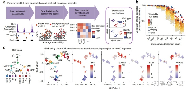
chromVAR是一个R包，用于分析单细胞或者bulk ATAC 或者DNAse-seq数据中染色质分析，作者在原文中提到这个R包通过预测染色质开放或者关闭（bam files）以及具有相同motif或者annotation的peaks（peak bed file）进而对染色质开放程度进行分析，同时这个R包也控制了技术误差。chromVAR的一个优点就是可以处理scATAC-seq数据。（但是我想处理的是bulk data所以就没有做cluster单细胞的聚类。）

贴上原文作者的话：（有点蠢，想了很久这句话的语法。。。）

analyzing sparse chromatin-accessibility data by estimating gain or loss of accessibility within peaks sharing the same motif or annotation while controlling for technical biases. chromVAR enables accurate clustering of scATAC-seq profiles and characterization of known andde novo sequence motifs associated with variation in chromatin accessibility.

2.安装

安装chromVAR需要用到BiocManager，大部分是BiocManager就可以下载的。

if (!requireNamespace("BiocManager", quietly = TRUE))
    install.packages("BiocManager")
BiocManager::install("chromVAR")

另外。作者还推荐了两个用vignettes下载的安装包以及一个github安装的包：

Two additional packages that are recommended and used in the vignettes:

motifmatchr - available on GitHub or development version of Bioconductor
JASPAR2016 - available from Bioconductor
Additionally, the package chromVARmotifs can be useful for loading additional motif collections:

chromVARmotifs - available on GitHub
devtools::install_github("GreenleafLab/chromVARmotifs")

运行chromVAR之前，作者建议用BiocParallel中register这个功能来确保可以并行操作。

For unix systems,

library(BiocParallel)
register(MulticoreParam(8)) # Use 8 cores

Windows系统的话，MulticoreParam是不能用的，但是可以用SnowParam:（同学教我的时候发现我这些都知道，他惊呆了……他以为我什么都不知道。。。）

register(SnowParam(SnowParam(workers=1, type = "SOCK")))

如果不想用超过单核的系统来跑的话，可以使用SerialParam:

register(SerialParam())

想了解register这个功能的话可以读一下BiocParallel里面的说明以及多核操作的一些options

3.输入数据

ChromVAR 包的输入数据包括3个：
1）比对后的reads bam file（或者bam bai也行）
2）chromatin accessibility peaks；（我用的是merged的narrowpeak或者peak.bed也行，）
3）一组代表motif位置的权重矩阵（PWM）或基因组注释的染色质特征数据集（这个地方我用的是chromVAR里的chromVARmotifs）

4.流程：

• 首先计算Raw deviation in accessibility
• 计算Raw deviation for background peaks
• Bias corrected deviations and z-scores
• motif heatmap plot

5.应用

先加载（Download package 到想哭）

library(data.table)
library(chromVAR)
library(motifmatchr)
library(SummarizedExperiment)
library(Matrix)
library(ggplot2)
library(BiocParallel)
library(BSgenome.Mmusculus.UCSC.mm10)
#这个地方我用的是mm10的，作者举例给的是hg19的，根据自己的情况来选吧
#这个包比较大，网络不稳定就直接bioconductor下载再install吧。

1.计算deviation（偏差）

针对于每一个motif和细胞，chromVAR都会首先计算这些样品map到peak上的片段数量间的差异以及期待的片段数量。（基于总的细胞平均值）
For each motif and cell, chromVAR first computes a ‘raw accessibility deviation’, the difference between the total number of fragments that map to peaks containing the motif and the expected number of fragments (based on the average of all cells).

在这一步需要load peak 文件和bam 文件，所以我们先load peak文件

peakfile <- "mypeaks.bed"（你的peak bed 文件）
peaks <- getPeaks(peakfile)（chromVAR 读取peak的功能）
#如果是narrowpeak的话，可以用下面这个,Iris是我的名字，请针对的改成你文件的名字呀。
readNarrowpeaks("Iris.narrowPeak")

再load bam文件

bamfiles <- c("mybam1.bam","mybam2.bam")

计算counts值。

fragment_counts <- getCounts(bamfiles, peaks, 
                              paired =  TRUE, 
                              by_rg = TRUE, 
                              format = "bam", 
                              colData = DataFrame(celltype = c("GM","K562")))

如果你现在没有数据的话，可以用作者的。有的话忽略这一行

data(example_counts, package = "chromVAR")

计算peaks中的GC含量（如果用作者的example，就把fragment_counts换成example_counts）

example_counts <- addGCBias(fragment_counts , 
                              genome = BSgenome.Mmusculus.UCSC.mm10)

过滤peak，默认的是non overlap还有最少有一个fragment匹配。

counts_filtered <- filterSamples(fragment_counts, min_depth = 1500,
                                  min_in_peaks = 0.15)
counts_filtered <- filterPeaks(counts_filtered)#过滤peaks，也有其他option.

2.match motif计算以及偏差计算

motifs <- getJasparMotifs()
motif_ix <- matchMotifs(motifs, counts_filtered,
                         genome = BSgenome.Mmusculus.UCSC.mm10)

# computing deviations（这一步计算很久）
dev <- computeDeviations(object = counts_filtered, 
                                 annotations = motif_ix)

ps：这一步computeDeviation计算需要很久，而且容易出现问题，我出现的问题是

'package:stats' may not be available when loading

对策是，google了一下发现这是Rstudio自己的问题，没理，继续往下进行。

以上是最基础的部分了，接下来就是应用和可视化了。

（以下代码和文字学习并摘抄自简书，前三个部分自己做了有一些tips，后续部分摘自简书作者六六，侵删。）

1.计算感兴趣的cell或样本之间每个motif或注释的变异性

variability <- computeVariability(dev)
plotVariability(variability, use_plotly = FALSE)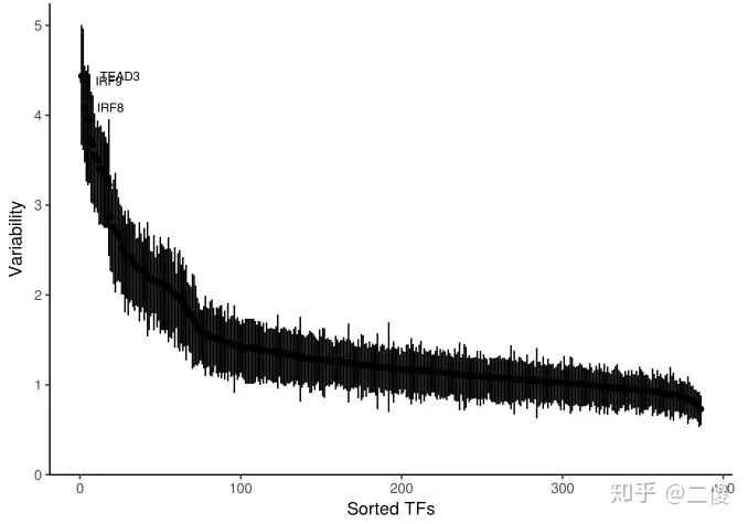

（这个图片引自简书，我自己画出来的variability不太好，很稀疏。）

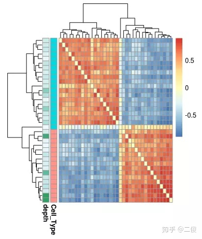
2.聚类

也可以用偏差校正偏差（bias corrected deviations）对样本聚类，函数getSampleCorrelation首先剔除高度相关注释和低可变性注释，然后细胞间的相关性。（其实我自己的代码，因为需要改变annotation名字以及需要polish，所以中间有很多小的代码没有放在这里了。）

library(pheatmap)
#因为之前画基因表达值的heatmap时总出现Inf问题，导致我有点心理阴影
sample_cor <- getSampleCorrelation(dev)

library(pheatmap)
pheatmap(as.dist(sample_cor), 
         annotation_row = colData(dev), 
         clustering_distance_rows = as.dist(1-sample_cor), 
         clustering_distance_cols = as.dist(1-sample_cor))

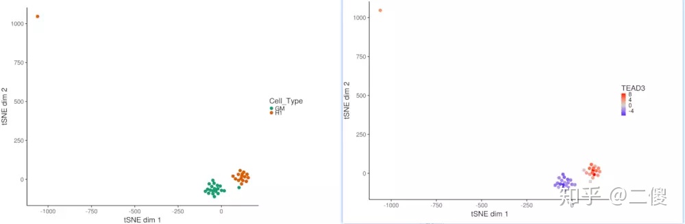
3.细胞或样本间的相似性

也可以用tSNE看细胞的相似性，函数deviationsTsne可以实现此功能。参数shiny=TRUE可以首先交互界面，perplexity根据细胞的实际数目调整，通常情况下，100个细胞时，perplexity在30-50都是可以的。

tsne_results <- deviationsTsne(dev, threshold = 1.5, perplexity = 10, 
                               shiny = FALSE)
# plotDeviationsTsne 绘图
tsne_plots <- plotDeviationsTsne(dev, tsne_results, #annotation = "TEAD3", 
                                   sample_column = "Cell_Type", shiny = FALSE)
#注意sample_column 名字要和colData中你的colname对应上。
tsne_plots[[1]]
tsne_plots[[2]]
#如果是画了注释和细胞分类的话就会有两个，可以输入tsne_plots来查看

ps：这个地方我搜了一下Perplexity的意思（因为我在设置10的时候，报错提醒我设置太高，所以查了一下，不是很懂，有不足请指正。）

信息论中，困惑度度量概率分布或概率模型的预测结果与样本的契合程度，困惑度越低则契合越准确。该度量可以用于比较不同模型之优劣。

（自己的结果聚类不太好，是sample PCA，所以还是放别人的图）

4.可及性和变异性的差异
函数differentialDeviations和differentialVariability可以看各组间对某一注释的偏差校正偏差是否存在显著性差异和显著性变异

diff_acc <- differentialDeviations(dev, "Cell_Type")
head(diff_acc)
##                           p_value p_value_adjusted
## MA0025.1_NFIL3       6.667785e-02     1.175006e-01
## MA0030.1_FOXF2       1.802723e-02     4.166773e-02
## MA0031.1_FOXD1       3.825026e-03     1.077708e-02

5. motif/kmer的相似性
设置参数what= "annotations"就可以用tsne看motif间的相似性

inv_tsne_results <- deviationsTsne(dev, threshold = 1.5, perplexity = 8, 
                                    what = "annotations", shiny = FALSE)
ggplot(inv_tsne_results, aes(x = Dim1, y = Dim2)) + geom_point() + 
  chromVAR_theme()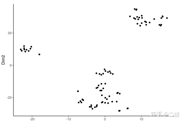

6. Kmers and sequence specificity of variation
利用kmers作为注释，我们可以使用kmers来识别染色质可及性变异所需的精确核苷酸。

kmer_ix <- matchKmers(6, counts_filtered, genome = BSgenome.Hsapiens.UCSC.hg19)
kmer_dev <- computeDeviations(counts_filtered, kmer_ix)
kmer_cov <- deviationsCovariability(kmer_dev)
plotKmerMismatch("CATTCC",kmer_cov)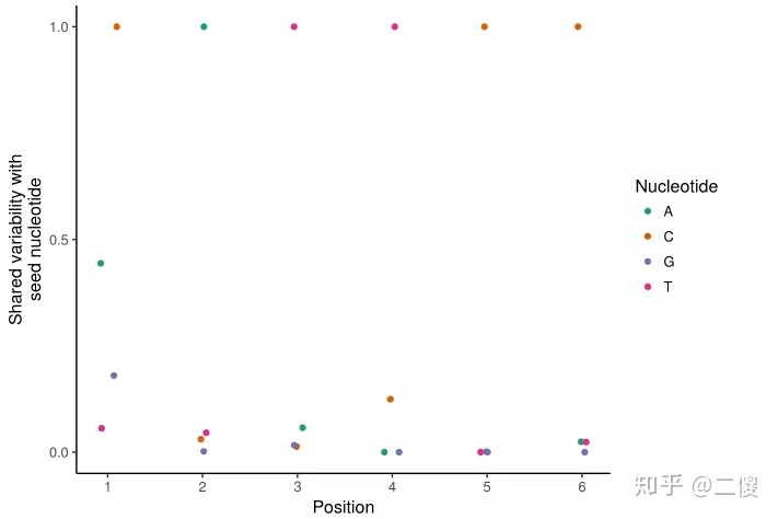

7. kmer从头组装
根据kmer偏差结果，可以使用assembleKmers函数构建de novo motif。

de_novos <- assembleKmers(kmer_dev, progress = FALSE) #no progress bar
de_novos

pwmDistance函数可以看de novo motif与已知motif的匹配关系，最终会返回3个列表，dist是每对motifs间的距离，strandmotif匹配的链，offset是motifs间的偏移。

dist_to_known <- pwmDistance(de_novos, motifs)
closest_match1 <- which.min(dist_to_known$dist[1,])
dist_to_known$strand[1,closest_match1]

library(ggmotif) # Package on github at AliciaSchep/ggmotif. Can use seqLogo alternatively
library(TFBSTools)
# De novo motif
ggmotif_plot(de_novos[[1]])
# Closest matching known
ggmotif_plot(toPWM(reverseComplement(motifs[[closest_match1]]),type = "prob"))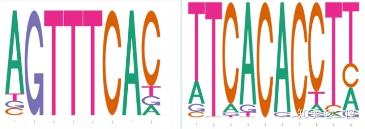

• 8. motif之间的协同作用
  chromVAR还包括计算注释/motif对之间“协同作用”的函数。

 getAnnotationSynergy(counts_filtered, motif_ix[,c(83,24,20)])
 

• 9. 相关性
  一个极端的协同值表明转录因子间可能存在合作或竞争的作用。函数getAnnotationCorrelation可以计算motifs间的相关性。

getAnnotationCorrelation(counts_filtered, motif_ix[,c(83,24,20)])

前两天有看到除了chromVAR之外，还有esATAC， ATAC-pipe也可以做ATAC-seq的分析，大概的走了一遍流程了解的多了一些，自己的数据分析完结果有点不太理想，会继续进行分析，很多地方可能写的不是很清楚，第一次做整理，有很多图片摘自简书作者六六，第一次学习也是根据他的文章，结合了作者简易的源代码和论文，如有不清楚或者不对的地方，请批评指正。