跟着Cell学单细胞转录组分析(十二):转录因子分析

转录因子分析可以了解细胞异质性背后的基因调控网络的异质性。转录因子分析也是单细胞转录组常见的分析内容，R语言分析一般采用的是SCENIC包，具体原理可参考两篇文章。1、《SCENIC : single-cell regulatory networkinference and clustering》。2、《Ascalable SCENIC workflow for single-cell gene regulatory network analysis》。但是说在前头，SCENIC的计算量超级大，非常耗费内存和时间，如非必要，不要用一般的电脑分析尝试。可以借助服务器完成分析，或者减少分析细胞数，再或者使用SCENIC的Python版本。这里我们也是仅仅进行演示，数据没有实际意义，人为减少了基因与细胞，然而就这也很费时间。重要的是看看流程。

首先开始前，需要做两件事。第一毫无疑问是安装和加载R包，需要的比较多，如果没有请安装。第二则是下载基因注释配套数据库。

library(Seurat)
library(tidyverse)
library(foreach)
library(RcisTarget)
library(doParallel)
library(SCopeLoomR)
library(AUCell)
BiocManager::install(c("doMC", "doRNG"))
library(doRNG)
BiocManager::install("GENIE3")
library(GENIE3)
#if (!requireNamespace("devtools", quietly = TRUE)) 
devtools::install_github("aertslab/SCENIC") 
packageVersion("SCENIC")
library(SCENIC)
#这里下载人的
dbFiles <- c("https://resources.aertslab.org/cistarget/databases/homo_sapiens/hg19/refseq_r45/mc9nr/gene_based/hg19-500bp-upstream-7species.mc9nr.feather",
             "https://resources.aertslab.org/cistarget/databases/homo_sapiens/hg19/refseq_r45/mc9nr/gene_based/hg19-tss-centered-10kb-7species.mc9nr.feather")
for(featherURL in dbFiles)
{
  download.file(featherURL, destfile=basename(featherURL)) 
}

接着就是构建分析文件。

#构建分析数据
exprMat <- as.matrix(immune@assays$RNA@data)#表达矩阵
exprMat[1:4,1:4]#查看数据
cellInfo <- immune@meta.data[,c("celltype","nCount_RNA","nFeature_RNA")]
colnames(cellInfo) <- c('CellType', 'nGene' ,'nUMI')
head(cellInfo)
table(cellInfo$CellType)
#构建scenicOptions对象，接下来的SCENIC分析都是基于这个对象的信息生成的
scenicOptions <- initializeScenic(org = "hgnc", dbDir = "F:/cisTarget_databases", nCores = 1)

构建共表达网络，最后一步很费时间。

# Co-expression network
genesKept <- geneFiltering(exprMat, scenicOptions)
exprMat.filtered <- exprMat[genesKept, ]
exprMat.filtered[1:4,1:4]
runCorrelation(exprMat.filtered, scenicOptions)
exprMat.filtered.log <- log2(exprMat.filtered + 1)
runGenie3(exprMat.filtered.log, scenicOptions)
#Using 676 TFs as potential regulators...
#Running GENIE3 part 1
#Running GENIE3 part 10
#Running GENIE3 part 2
#Running GENIE3 part 3
#Running GENIE3 part 4
#Running GENIE3 part 5
#Running GENIE3 part 6
#Running GENIE3 part 7
#Running GENIE3 part 8
#Running GENIE3 part 9
#Finished running GENIE3.
#Warning message:
#In runGenie3(exprMat.filtered.log, scenicOptions) :
#  Only 676 (37%) of the 1839 TFs in the database were found in the dataset. Do they use the same gene IDs?

构建基因调控网络GRN并进行AUC评分。也是耗费时间的过程。运行完成的结果就是整个分析得到的内容，需要按照自己的目的去筛选。

# Build and score the GRN
scenicOptions <- runSCENIC_1_coexNetwork2modules(scenicOptions)
scenicOptions <- runSCENIC_2_createRegulons(scenicOptions)
exprMat_log <- log2(exprMat + 1)
scenicOptions <- runSCENIC_3_scoreCells(scenicOptions,exprMat_log)
scenicOptions <- runSCENIC_4_aucell_binarize(scenicOptions)
saveRDS(scenicOptions, file = "int/scenicOptions.Rds")

以下是运行记录

>scenicOptions <- runSCENIC_2_createRegulons(scenicOptions)
13:21  Step 2. Identifying regulons
tfModulesSummary:
                        [,1]
top5perTargetAndtop3sd     1
top5perTargetAndtop50      1
top1sdAndtop10perTarget    2
top50perTargetAndtop1sd    2
top50Andtop10perTarget     3
w0.005                    27
w0.005Andtop1sd          149
top50perTarget           174
top50Andtop3sd           236
top3sd                   436
top50                    436
w0.005Andtop50perTarget  500
top1sd                   523
top5perTarget            617
top10perTarget           671
w0.001                   676
13:21  RcisTarget: Calculating AUC
Scoring database:  [Source file: hg19-500bp-upstream-7species.mc9nr.feather]
Scoring database:  [Source file: hg19-tss-centered-10kb-7species.mc9nr.feather]
Not all characters in C:/Users/liuhl/Desktop/1.R could be decoded using CP936. To try a different encoding, choose "File | Reopen with Encoding..." from the main menu.17:17  RcisTarget: Adding motif annotation
Using BiocParallel...
Using BiocParallel...
Number of motifs in the initial enrichment: 1993247
Number of motifs annotated to the matching TF: 22290
17:38  RcisTarget: Pruning targets
19:04  Number of motifs that support the regulons: 12551
  Preview of motif enrichment saved as: output/Step2_MotifEnrichment_preview.html
There were 13 warnings (use warnings() to see them)
> exprMat_log <- log2(exprMat + 1)
> scenicOptions <- runSCENIC_3_scoreCells(scenicOptions,exprMat_log)
19:06  Step 3. Analyzing the network activity in each individual cell
  Number of regulons to evaluate on cells: 318
Biggest (non-extended) regulons: 
   ELF1 (1760g)
   ETS1 (1734g)
   FLI1 (1604g)
   ELK3 (1493g)
   POLR2A (1453g)
   CHD2 (1251g)
   ETV3 (1249g)
   ELK4 (1148g)
   TAF1 (974g)
   ERG (956g)
Quantiles for the number of genes detected by cell: 
(Non-detected genes are shuffled at the end of the ranking. Keep it in mind when choosing the threshold for calculating the AUC).
   min     1%     5%    10%    50%   100% 
205.00 224.76 276.90 321.40 695.00 997.00 
Warning in .AUCell_calcAUC(geneSets = geneSets, rankings = rankings, nCores = nCores,  :
  Using only the first 224.76 genes (aucMaxRank) to calculate the AUC.
19:07  Finished running AUCell.
19:07  Plotting heatmap...
19:07  Plotting t-SNEs...
Warning message:
In max(densCurve$y[nextMaxs]) : max里所有的参数都不存在；回覆-Inf
> scenicOptions <- runSCENIC_4_aucell_binarize(scenicOptions)
Binary regulon activity: 207 TF regulons x 439 cells.
(299 regulons including 'extended' versions)
168 regulons are active in more than 1% (4.39) cells.
> saveRDS(scenicOptions, file = "int/scenicOptions.Rds")

每一步的分析结果SCENIC都会自动保存在所创建的int和out文件夹。接下来对结果进行可视化，这里是随机选的，没有生物学意义。实际情况是要根据自己的研究目的。

1、可视化转录因子与seurat细胞分群联动

#regulons AUC
AUCmatrix <- readRDS("int/3.4_regulonAUC.Rds")
AUCmatrix <- AUCmatrix@assays@data@listData$AUC
AUCmatrix <- data.frame(t(AUCmatrix), check.names=F)
RegulonName_AUC <- colnames(AUCmatrix)
RegulonName_AUC <- gsub(' \\(','_',RegulonName_AUC)
RegulonName_AUC <- gsub('\\)','',RegulonName_AUC)
colnames(AUCmatrix) <- RegulonName_AUC
scRNAauc <- AddMetaData(immune, AUCmatrix)
scRNAauc@assays$integrated <- NULL
saveRDS(scRNAauc,'immuneauc.rds')

#二进制regulo AUC
BINmatrix <- readRDS("int/4.1_binaryRegulonActivity.Rds")
BINmatrix <- data.frame(t(BINmatrix), check.names=F)
RegulonName_BIN <- colnames(BINmatrix)
RegulonName_BIN <- gsub(' \\(','_',RegulonName_BIN)
RegulonName_BIN <- gsub('\\)','',RegulonName_BIN)
colnames(BINmatrix) <- RegulonName_BIN
scRNAbin <- AddMetaData(immune, BINmatrix)
scRNAbin@assays$integrated <- NULL
saveRDS(scRNAbin, 'immunebin.rds')

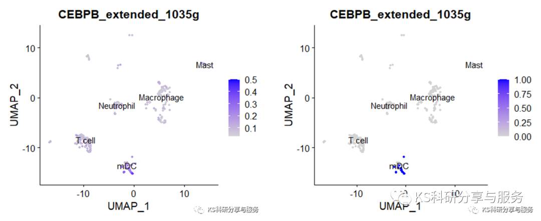
作图使用Seurat中FeaturePlot函数。小提琴图也是可以的。

FeaturePlot(scRNAauc, features='CEBPB_extended_1035g', label=T, reduction = 'umap')
FeaturePlot(scRNAbin, features='CEBPB_extended_1035g', label=T, reduction = 'umap')

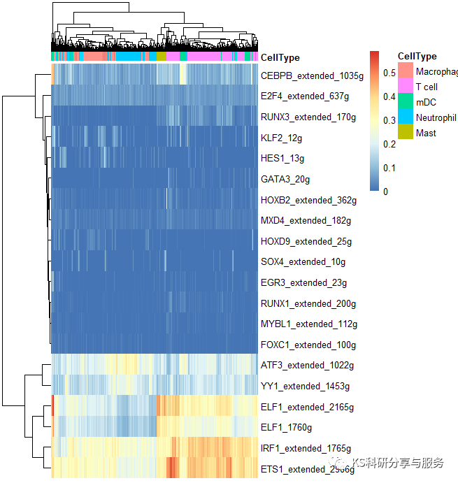
2、最常见的热图，选择需要可视化的regulons。

library(pheatmap)
celltype = subset(cellInfo,select = 'CellType')
AUCmatrix <- t(AUCmatrix)
BINmatrix <- t(BINmatrix)
regulons <- c('CEBPB_extended_1035g','RUNX1_extended_200g',
                 'FOXC1_extended_100g','MYBL1_extended_112g',
                 'IRF1_extended_1785g',
                 'ELF1_1760g','ELF1_extended_2165g',
                 'IRF1_extended_1765g','ETS1_extended_2906g',
                 'YY1_extended_1453g','ATF3_extended_1022g',
                 'E2F4_extended_637g',
                 'KLF2_12g','HES1_13g',
                 'GATA3_20g','HOXB2_extended_362g',
                 'SOX4_extended_10g',
                 'RUNX3_extended_170g','EGR3_extended_23g',
                 'MXD4_extended_182g','HOXD9_extended_25g')
AUCmatrix <- AUCmatrix[rownames(AUCmatrix)%in%regulons,]
BINmatrix <- BINmatrix[rownames(BINmatrix)%in%regulons,]
pheatmap(AUCmatrix, show_colnames=F, annotation_col=celltype,
         width = 6, height = 5)
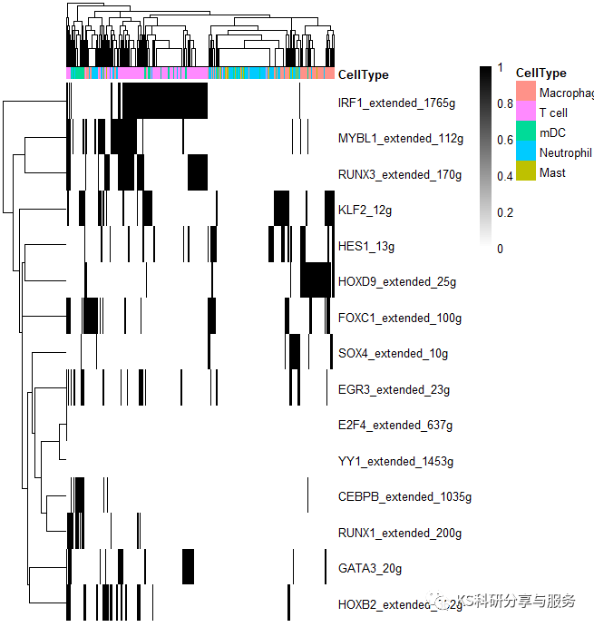
pheatmap(BINmatrix, show_colnames=F, annotation_col=celltype,
         color = colorRampPalette(colors = c("white","black"))(100),
         width = 6, height = 5)

好了，以上是一个基本的流程演示，具体怎么用这个结果，如何解读，可以参考相关的高分文献，了解分析原理，与自己的研究相结合。
更多精彩内容请访问我的个人公众号《KS科研分享与服务》！