卷积中的attention map理解及可视化

最新推荐文章于 2024-05-27 18:52:42 发布

颐水风华

最新推荐文章于 2024-05-27 18:52:42 发布

阅读量2.9w

点赞数 9

分类专栏：网络架构

网络架构专栏收录该内容

18 篇文章 0 订阅

订阅专栏

引用
Woo S , Park J , Lee J Y , et al. CBAM: Convolutional Block Attention Module[J]. 2018.
下载
https://arxiv.org/pdf/1807.06521.pdf
转载于：
https://www.jianshu.com/p/4fac94eaca91
https://blog.csdn.net/weixin_36541072/article/details/79126225

摘要

论文提出了Convolutional Block Attention Module(CBAM)，这是一种为卷积神将网络设计的，简单有效的注意力模块(Attention Module)。对于卷积神经网络生成的feature map，CBAM从通道和空间两个维度计算feature map的attention map，然后将attention map与输入的feature map相乘来进行特征的自适应学习。CBAM是一个轻量的通用模块，可以将其融入到各种卷积神经网络中进行端到端的训练。

主要思想

对于一个中间层的feature map： $F \in\mathbb R^{C*H*W}$ ，CBAM将会顺序推理出1维的channel attention map $M_c \in\mathbb R^{C*1*1}$ 以及2维的spatial attention map $M_s \in\mathbb R^{1*H*W}$ ，整个过程如下所示：

$F^{'} = M_c(F) \otimes F$

$F^{''}=M_s(F^{'}) \otimes F^{'}$

其中 $\otimes$ 为element-wise multiplication，首先将channel attention map与输入的feature map相乘得到 $F^{'}$ ，之后计算 $F^{'}$ 的spatial attention map，并将两者相乘得到最终的输出 $F^{''}$ 。下图为CBAM的示意图：

CBAM的结构图

Channel attention module

feature map 的每个channel都被视为一个feature detector，channel attention主要关注于输入图片中什么(what)是有意义的。为了高效地计算channel attention，论文使用最大池化和平均池化对feature map在空间维度上进行压缩，得到两个不同的空间背景描述： $F^{c}_{max}$ 和 $F^{c}_{avg}$ 。使用由MLP组成的共享网络对这两个不同的空间背景描述进行计算得到channel attention map： $M_c \in\mathbb R^{C*1*1}$ 。计算过程如下：

$M_c(F) = \sigma(MLP(AvgPool(F)) + MLP(MaxPool(F)))$

$M_c(F) = \sigma(W_1(W_0(F^{c}_{avg})) + W_1(W_0(F^{c}_{max})))$

其中 $W_0 \in \mathbb R^{C/r * C}$ ， $W_1 \in \mathbb R^{C * C/r}$ ， $W_0$ 后使用了Relu作为激活函数。

Spatial attention module.

与channel attention不同，spatial attention主要关注于位置信息(where)。为了计算spatial attention，论文首先在channel的维度上使用最大池化和平均池化得到两个不同的特征描述 $F^{s}_{max} \in \mathbb R_{1*H*W}$ 和 $F^{s}_{avg} \in \mathbb R_{1*H*W}$ ，然后使用concatenation将两个特征描述合并，并使用卷积操作生成spatial attention map $M_s(F) \in \mathbb R_{H*W}$ 。计算过程如下：

$M_s(F) = \sigma(f^{7*7}([AvgPool(F); MaxPool(F)]))$

$M_s(F) = \sigma(f^{7*7}([F^{s}_{avg}; F^{s}_{max}]))$

其中， $f^{7*7}$ 表示7*7的卷积层

下图为channel attention和spatial attention的示意图：

（上）channel attention module；（下）spatial attention module

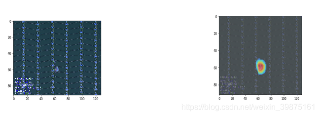
简单了说：通过深度学习的方法，自动判defect类型。并画出attention map。找到其中的defect位置，就可以不用Rcnn等方法去标记bbox。

代码实现tensorflow 1.9

"""
@Time   : 2018/10/19
@Author : Li YongHong
@Email  : lyh_robert@163.com
@File   : test.py
"""
import tensorflow as tf
import numpy as np

slim = tf.contrib.slim

def combined_static_and_dynamic_shape(tensor):
  """Returns a list containing static and dynamic values for the dimensions.

  Returns a list of static and dynamic values for shape dimensions. This is
  useful to preserve static shapes when available in reshape operation.

  Args:
    tensor: A tensor of any type.

  Returns:
    A list of size tensor.shape.ndims containing integers or a scalar tensor.
  """
  static_tensor_shape = tensor.shape.as_list()
  dynamic_tensor_shape = tf.shape(tensor)
  combined_shape = []
  for index, dim in enumerate(static_tensor_shape):
    if dim is not None:
      combined_shape.append(dim)
    else:
      combined_shape.append(dynamic_tensor_shape[index])
  return combined_shape

def convolutional_block_attention_module(feature_map, index, inner_units_ratio=0.5):
    """
    CBAM: convolution block attention module, which is described in "CBAM: Convolutional Block Attention Module"
    Architecture : "https://arxiv.org/pdf/1807.06521.pdf"
    If you want to use this module, just plug this module into your network
    :param feature_map : input feature map
    :param index : the index of convolution block attention module
    :param inner_units_ratio: output units number of fully connected layer: inner_units_ratio*feature_map_channel
    :return:feature map with channel and spatial attention
    """
    with tf.variable_scope("cbam_%s" % (index)):
        feature_map_shape = combined_static_and_dynamic_shape(feature_map)
        # channel attention
        channel_avg_weights = tf.nn.avg_pool(
            value=feature_map,
            ksize=[1, feature_map_shape[1], feature_map_shape[2], 1],
            strides=[1, 1, 1, 1],
            padding='VALID'
        )
        channel_max_weights = tf.nn.max_pool(
            value=feature_map,
            ksize=[1, feature_map_shape[1], feature_map_shape[2], 1],
            strides=[1, 1, 1, 1],
            padding='VALID'
        )
        channel_avg_reshape = tf.reshape(channel_avg_weights,
                                         [feature_map_shape[0], 1, feature_map_shape[3]])
        channel_max_reshape = tf.reshape(channel_max_weights,
                                         [feature_map_shape[0], 1, feature_map_shape[3]])
        channel_w_reshape = tf.concat([channel_avg_reshape, channel_max_reshape], axis=1)

        fc_1 = tf.layers.dense(
            inputs=channel_w_reshape,
            units=feature_map_shape[3] * inner_units_ratio,
            name="fc_1",
            activation=tf.nn.relu
        )
        fc_2 = tf.layers.dense(
            inputs=fc_1,
            units=feature_map_shape[3],
            name="fc_2",
            activation=None
        )
        channel_attention = tf.reduce_sum(fc_2, axis=1, name="channel_attention_sum")
        channel_attention = tf.nn.sigmoid(channel_attention, name="channel_attention_sum_sigmoid")
        channel_attention = tf.reshape(channel_attention, shape=[feature_map_shape[0], 1, 1, feature_map_shape[3]])
        feature_map_with_channel_attention = tf.multiply(feature_map, channel_attention)
        # spatial attention
        channel_wise_avg_pooling = tf.reduce_mean(feature_map_with_channel_attention, axis=3)
        channel_wise_max_pooling = tf.reduce_max(feature_map_with_channel_attention, axis=3)

        channel_wise_avg_pooling = tf.reshape(channel_wise_avg_pooling,
                                              shape=[feature_map_shape[0], feature_map_shape[1], feature_map_shape[2],
                                                     1])
        channel_wise_max_pooling = tf.reshape(channel_wise_max_pooling,
                                              shape=[feature_map_shape[0], feature_map_shape[1], feature_map_shape[2],
                                                     1])

        channel_wise_pooling = tf.concat([channel_wise_avg_pooling, channel_wise_max_pooling], axis=3)
        spatial_attention = slim.conv2d(
            channel_wise_pooling,
            1,
            [7, 7],
            padding='SAME',
            activation_fn=tf.nn.sigmoid,
            scope="spatial_attention_conv"
        )
        feature_map_with_attention = tf.multiply(feature_map_with_channel_attention, spatial_attention)
        return feature_map_with_attention

#example
feature_map = tf.constant(np.random.rand(2,8,8,32), dtype=tf.float16)
feature_map_with_attention = convolutional_block_attention_module(feature_map, 1)

with tf.Session() as sess:
    init = tf.global_variables_initializer()
    sess.run(init)
    result = sess.run(feature_map_with_attention)
    print(result.shape)

kears的map

https://github.com/datalogue/keras-attention/blob/master/visualize.py

attention map可视化

下面开始抄另一个人的

1. 卷积知识补充

为了后面方便讲解代码，这里先对卷积的部分知识进行一下简介。关于卷积核如何在图像的一个通道上进行滑动计算，网上有诸多资料，相信对卷积神经网络有一定了解的读者都应该比较清楚，本文就不再赘述。这里主要介绍一组卷积核如何在一幅图像上计算得到一组feature map。

以从原始图像经过第一个卷积层得到第一组feature map为例（从得到的feature map到再之后的feature map也是同理），假设第一组feature map共有64个，那么可以把这组feature map也看作一幅图像，只不过它的通道数是64，而一般意义上的图像是RGB3个通道。为了得到这第一组feature map，我们需要64个卷积核，每个卷积核是一个k x k x 3的矩阵，其中k是卷积核的大小（假设是正方形卷积核），3就对应着输入图像的通道数。下面我以一个简单粗糙的图示来展示一下图像经过一个卷积核的卷积得到一个feature map的过程。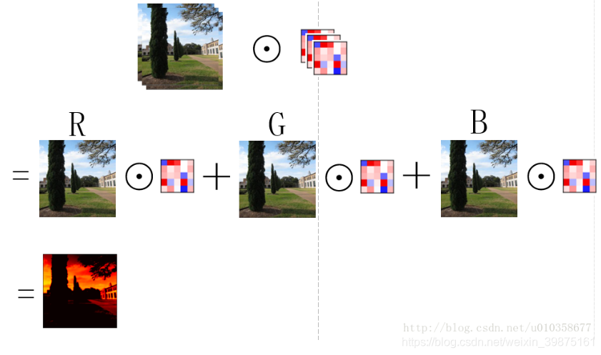

如图所示，其实可以看做卷积核的每一通道（不太准确，将就一下）和图像的每一通道对应进行卷积操作，然后再逐位置相加，便得到了一个feature map。

那么用一组（64个）卷积核去卷积一幅图像，得到64个feature map就如下图所示，也就是每个卷积核得到一个feature map，64个卷积核就得到64个feature map。
group_conv

另外，也可以稍微换一个角度看待这个问题，那就是先让图片的某一通道分别与64个卷积核的对应通道做卷积，得到64个feature map的中间结果，之后3个通道对应的中间结果再相加，得到最终的feature map，如下图所示：

conv2

可以看到这其实就是第一幅图扩展到多卷积核的情形，图画得较为粗糙，有些中间结果和最终结果直接用了一样的子图，理解时请稍微注意一下。下面代码中对卷积核进行展示的时候使用的就是这种方式，即对应着输入图像逐通道的去显示卷积核的对应通道，而不是每次显示一个卷积核的所有通道，可能解释的有点绕，需要注意一下。通过下面这个小图也许更好理解。
box

颐水风华

关注

9
点赞
踩
70

收藏

觉得还不错? 一键收藏
3
评论
卷积中的attention map理解及可视化

引用Woo S , Park J , Lee J Y , et al. CBAM: Convolutional Block Attention Module[J]. 2018.下载https://arxiv.org/pdf/1807.06521.pdf转载于：https://www.jianshu.com/p/4fac94eaca91https://blog.csdn.net/wei...
复制链接

扫一扫