【OpenMMLab实践】01MMSegmentation官方教程实现过程记录（mmcv，mmsegmentation，torch）

本文主要根据mmsegmentation的官方教程（教程链接在这里），并且看了b站的视频，一步步实现代码中的demo教程，主要包含以下两方面的功能：

• 通过MMSeg加载预训练好的权重，输入单张图片，实现分割，并可视化分割图
• 自定义数据集，修改配置文件，重新训练模型，并可视化分割图

1. 编程环境准备

1.1 检查平台上pytorch版本

# step1:检查平台上PyTorch版本，在终端输入此命令
!pip list | grep torch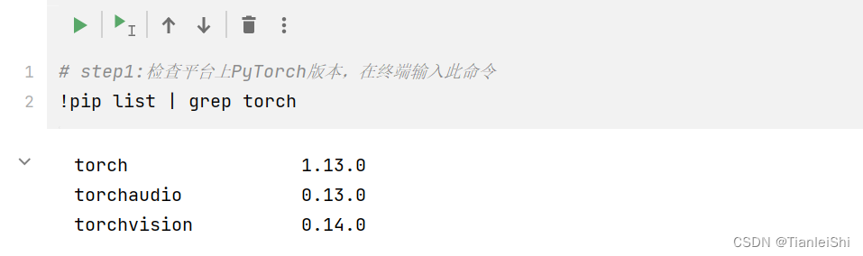

1.2 检查torch以及gpu是否可用

import torch
num_gpu = torch.cuda.device_count()
device = torch.device('cuda:0' if (torch.cuda.is_available() and num_gpu>0) else 'cpu')
print('Number of gpu:{}\nDevice:{}'.format(num_gpu,device))
torch.cuda.get_device_name(0)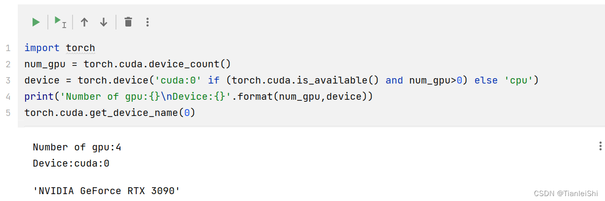

 

 1.3 安装mmcv第三方库

该过程可参考官方安装教程，注意版本的匹配

1.4 通过源码安装mmsegmentation程序

首先创建一个文件夹OpenMMLab_My

%cd ./OpemMMLab_My
!rm -rf mmsegmentation
!git clone https://github.com/open-mmlab/mmsegmentation.git
%cd mmsegmentation
!pip install -e .

1.5 最后检查一下mmseg是否安装成功

# Check Pytorch installation
import torch,torchvision
print(torch.__version__,torch.cuda.is_available())

# Check MMSegmentation installation
import mmseg
print(mmseg.__version__)

1.13.0 True
0.29.1

2. 使用预训练的分割模型实现测试

2.1 下载PSPNet预训练模型

# 从Model Zooo 获取PSPNet预训练模型的链接，下载并保存在checkpoints文件夹中
!mkdir checkpoints
!wget https://download.openmmlab.com/mmsegmentation/v0.5/pspnet/pspnet_r50-d8_512x1024_40k_cityscapes/pspnet_r50-d8_512x1024_40k_cityscapes_20200605_003338-2966598c.pth -P checkpoints

 2.2 设置配置文件路径和模型参数文件路径

# 设置配置文件和参数文件路径
# config_file = 'configs/pspnet/pspnet_r50-d8_512x1024_40k_cityscapes.py'
config_file = "/home/shitianlei/OpenMMLab_My/mmsegmentation/configs/pspnet/pspnet_r50-d8_512x1024_40k_cityscapes.py"
checkpoint_file = 'checkpoints/pspnet_r50-d8_512x1024_40k_cityscapes_20200605_003338-2966598c.pth'

2.4 加载图像并进行推理

# 使用Python API 构建模型
import mmcv
from mmseg.apis import init_segmentor
model = init_segmentor(config_file,checkpoint_file,device='cuda:0')
img = 'demo.png'
img_img = mmcv.imread(img)
print(img_img.shape)
result = inference_segmentor(model,img)

2.5 通过show_result_pyplot接口可视化分割结果

# 可视化分割图
show_result_pyplot(model, img, result, get_palette('cityscapes'))

 2.6 为每一种颜色创建图例

from mmseg.datasets import CityscapesDataset
import numpy as np
import mmcv
from PIL import Image
# 获取类别名和调色板
classes = CityscapesDataset.CLASSES
palette = CityscapesDataset.PALETTE

# 将分割图按调色板染色
seg_map = result[0].astype('uint8')
seg_img = Image.fromarray(seg_map).convert('P')
seg_img.putpalette(np.array(palette,dtype=np.uint8))

from matplotlib import pyplot as plt
import matplotlib.patches as mpatches
plt.figure(figsize=(14,8))

print(seg_map.shape)
im = plt.imshow(((np.array(seg_img.convert('RGB')))*0.4 + mmcv.imread('demo.png')*0.6)/255)

# 为每一种颜色创建一个图例
patches = [mpatches.Patch(color = np.array(palette[i])/255.,label=classes[i]) for i in range(8)]
plt.legend(handles = patches,bbox_to_anchor=(1.05,1),loc=2,borderaxespad=0.,fontsize='large')
plt.show()

3. 在自定义数据集上训练分割模型

主要包含以下步骤：

• 增加一个新的数据集类型
• 修改对应配置文件
• 启动和测试

3.1 实现一个新的数据集类型

•  在MMSegmentation中Datasets要求图像和语义分割标注需要放在同意路径的文件夹下，所以为了支持新的数据集，我们需要修改最初的文件结构

• 官方提供了一个转换数据集的实例。详情参考如下链接：docs

• 这里使用了standfore background dataset作为示例。本数据集一共包含715张图像，主要是室外场景，每张图像的尺寸是320*240pixels

• 这里使用region annotations作为训练的标签。一共有8类，天空，树，路，草，水，建筑，山和前景。i.e. sky, tree, road, grass, water, building, mountain, and foreground object.

# download and unzip
!wget http://dags.stanford.edu/data/iccv09Data.tar.gz -O stanford_background.tar.gz
!tar xf stanford_background.tar.gz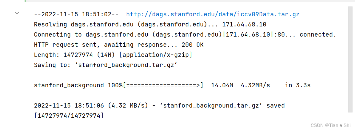

3.2 加载一张图像看看

# Let's take a look at the dataset
import mmcv
import matplotlib.pyplot as plt

img = mmcv.imread('iccv09Data/images/6000124.jpg')
plt.figure(figsize=(8, 6))
plt.imshow(mmcv.bgr2rgb(img))
plt.show()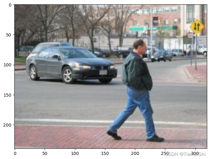

3.3 将标注文件转换成分割图

import os.path as osp
import numpy as np
from PIL import Image
# convert dataset annotation to semantic segmentation map
data_root = 'iccv09Data'
img_dir = 'images'
ann_dir = 'labels'
# define class and plaette for better visualization
classes = ('sky', 'tree', 'road', 'grass', 'water', 'bldg', 'mntn', 'fg obj')
palette = [[128, 128, 128], [129, 127, 38], [120, 69, 125], [53, 125, 34], 
           [0, 11, 123], [118, 20, 12], [122, 81, 25], [241, 134, 51]]
for file in mmcv.scandir(osp.join(data_root, ann_dir), suffix='.regions.txt'):
  seg_map = np.loadtxt(osp.join(data_root, ann_dir, file)).astype(np.uint8)
  seg_img = Image.fromarray(seg_map).convert('P')
  seg_img.putpalette(np.array(palette, dtype=np.uint8))
  seg_img.save(osp.join(data_root, ann_dir, file.replace('.regions.txt', 
                                                         '.png')))

3.4 加载一张mask看看

# Let's take a look at the segmentation map we got
import matplotlib.patches as mpatches
img = Image.open('iccv09Data/labels/6000124.png')
plt.figure(figsize=(8, 6))
im = plt.imshow(np.array(img.convert('RGB')))

# create a patch (proxy artist) for every color 为每一种颜色创建一个图例
patches = [mpatches.Patch(color=np.array(palette[i])/255., 
                          label=classes[i]) for i in range(8)]
# put those patched as legend-handles into the legend
plt.legend(handles=patches, bbox_to_anchor=(1.05, 1), loc=2, borderaxespad=0., 
           fontsize='large')

plt.show()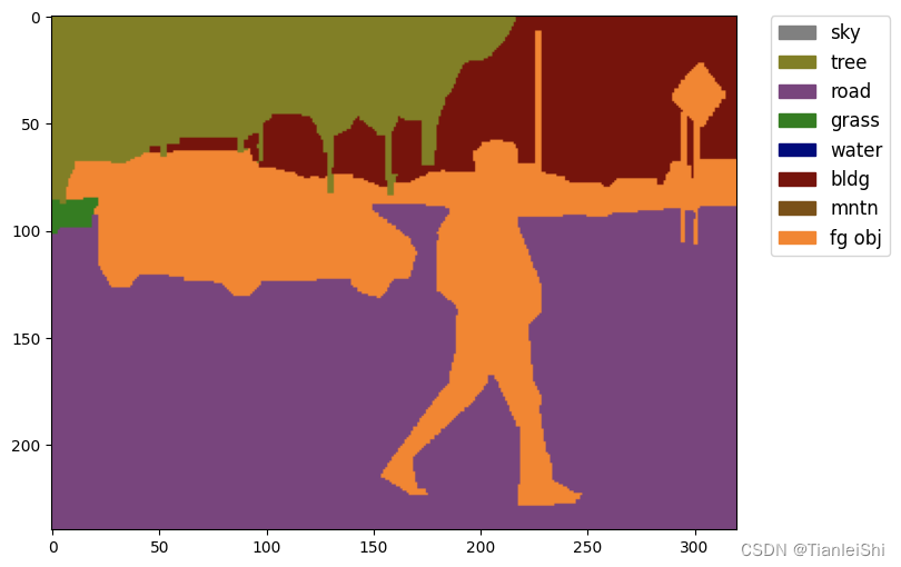

3.5 划分训练集和验证集

# split train/val set randomly
split_dir = 'splits'
mmcv.mkdir_or_exist(osp.join(data_root, split_dir))
filename_list = [osp.splitext(filename)[0] for filename in mmcv.scandir(
    osp.join(data_root, ann_dir), suffix='.png')]
with open(osp.join(data_root, split_dir, 'train.txt'), 'w') as f:
  # select first 4/5 as train set
  train_length = int(len(filename_list)*4/5)
  f.writelines(line + '\n' for line in filename_list[:train_length])
with open(osp.join(data_root, split_dir, 'val.txt'), 'w') as f:
  # select last 1/5 as train set
  f.writelines(line + '\n' for line in filename_list[train_length:])

3.6 修改数据集类

from mmseg.datasets.builder import DATASETS
from mmseg.datasets.custom import CustomDataset

@DATASETS.register_module()
class StanfordBackgroundDataset(CustomDataset):
  CLASSES = classes
  PALETTE = palette
  def __init__(self, split, **kwargs):
    super().__init__(img_suffix='.jpg', seg_map_suffix='.png', 
                     split=split, **kwargs)
    assert osp.exists(self.img_dir) and self.split is not None

3.7 创建配置文件

接下来，修改配置文件进行训练。为了加速训练过程，我们使用模型微调。

from mmcv import Config
cfg = Config.fromfile("/home/shitianlei/OpenMMLab_My/mmsegmentation/configs/pspnet/pspnet_r50-d8_512x1024_40k_cityscapes.py")

上面使用的配置文件是基于cityscapes数据集训练的PSPNet模型，我们需要根据我们的新的数据集对这个配置文件进行修改。

from mmseg.apis import set_random_seed
from mmseg.utils import get_device

# Since we use only one GPU, BN is used instead of SyncBN
cfg.norm_cfg = dict(type='BN', requires_grad=True)
cfg.model.backbone.norm_cfg = cfg.norm_cfg
cfg.model.decode_head.norm_cfg = cfg.norm_cfg
cfg.model.auxiliary_head.norm_cfg = cfg.norm_cfg
# modify num classes of the model in decode/auxiliary head
cfg.model.decode_head.num_classes = 8
cfg.model.auxiliary_head.num_classes = 8

# Modify dataset type and path
cfg.dataset_type = 'StanfordBackgroundDataset'
cfg.data_root = data_root

cfg.data.samples_per_gpu = 8
cfg.data.workers_per_gpu=8

cfg.img_norm_cfg = dict(
    mean=[123.675, 116.28, 103.53], std=[58.395, 57.12, 57.375], to_rgb=True)
cfg.crop_size = (256, 256)
cfg.train_pipeline = [
    dict(type='LoadImageFromFile'),
    dict(type='LoadAnnotations'),
    dict(type='Resize', img_scale=(320, 240), ratio_range=(0.5, 2.0)),#主要是修改图像尺寸
    dict(type='RandomCrop', crop_size=cfg.crop_size, cat_max_ratio=0.75),
    dict(type='RandomFlip', flip_ratio=0.5),
    dict(type='PhotoMetricDistortion'),
    dict(type='Normalize', **cfg.img_norm_cfg),
    dict(type='Pad', size=cfg.crop_size, pad_val=0, seg_pad_val=255),
    dict(type='DefaultFormatBundle'),
    dict(type='Collect', keys=['img', 'gt_semantic_seg']),
]

cfg.test_pipeline = [
    dict(type='LoadImageFromFile'),
    dict(
        type='MultiScaleFlipAug',
        img_scale=(320, 240),#主要是修改图像尺寸
        # img_ratios=[0.5, 0.75, 1.0, 1.25, 1.5, 1.75],
        flip=False,
        transforms=[
            dict(type='Resize', keep_ratio=True),
            dict(type='RandomFlip'),
            dict(type='Normalize', **cfg.img_norm_cfg),
            dict(type='ImageToTensor', keys=['img']),
            dict(type='Collect', keys=['img']),
        ])
]


cfg.data.train.type = cfg.dataset_type
cfg.data.train.data_root = cfg.data_root
cfg.data.train.img_dir = img_dir
cfg.data.train.ann_dir = ann_dir
cfg.data.train.pipeline = cfg.train_pipeline
cfg.data.train.split = 'splits/train.txt'

cfg.data.val.type = cfg.dataset_type
cfg.data.val.data_root = cfg.data_root
cfg.data.val.img_dir = img_dir
cfg.data.val.ann_dir = ann_dir
cfg.data.val.pipeline = cfg.test_pipeline
cfg.data.val.split = 'splits/val.txt'

cfg.data.test.type = cfg.dataset_type
cfg.data.test.data_root = cfg.data_root
cfg.data.test.img_dir = img_dir
cfg.data.test.ann_dir = ann_dir
cfg.data.test.pipeline = cfg.test_pipeline
cfg.data.test.split = 'splits/val.txt'

# We can still use the pre-trained Mask RCNN model though we do not need to
# use the mask branch
cfg.load_from = 'checkpoints/pspnet_r50-d8_512x1024_40k_cityscapes_20200605_003338-2966598c.pth'

# Set up working dir to save files and logs.
cfg.work_dir = './work_dirs/tutorial'

cfg.runner.max_iters = 200
cfg.log_config.interval = 10
cfg.evaluation.interval = 200
cfg.checkpoint_config.interval = 200

# Set seed to facitate reproducing the result
cfg.seed = 0
set_random_seed(0, deterministic=False)
cfg.gpu_ids = range(1)
cfg.device = get_device()

# Let's have a look at the final config used for training
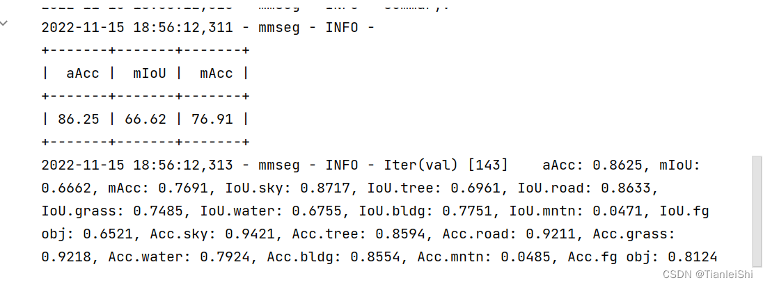
print(f'Config:\n{cfg.pretty_text}')

3.8 训练和评估

from mmseg.datasets import build_dataset
from mmseg.models import build_segmentor
from mmseg.apis import train_segmentor


# Build the dataset
datasets = [build_dataset(cfg.data.train)]

# Build the detector
model = build_segmentor(cfg.model)
# Add an attribute for visualization convenience
model.CLASSES = datasets[0].CLASSES

# Create work_dir
mmcv.mkdir_or_exist(osp.abspath(cfg.work_dir))
train_segmentor(model, datasets, cfg, distributed=False, validate=True, 
                meta=dict())

 3.9 图像推理

img = mmcv.imread('iccv09Data/images/6000124.jpg')

model.cfg = cfg
result = inference_segmentor(model, img)
plt.figure(figsize=(8, 6))
show_result_pyplot(model, img, result, palette)