小波分析（PyWavelets）

小波

安装库

conda activate PY3.7
pip install PyWavelets

使用

引入

import pywt

查看小波对应的名称

pywt.wavelist()

cwt

连续小波变换例子

(cwtmatr, frequencies)= pywt.cwt(S[1,16000:19000],scales=8,wavelet='mexh',sampling_period=1/250);

函数定义

pywt.cwt(data, scales, wavelet)
One dimensional Continuous Wavelet Transform.

Parameters:	
data : array_like
Input signal

scales : array_like
The wavelet scales to use. One can use f = scale2frequency(wavelet, scale)/sampling_period to determine what physical frequency, f. Here, f is in hertz when the sampling_period is given in seconds.

wavelet : Wavelet object or name
Wavelet to use

sampling_period : float
Sampling period for the frequencies output (optional). The values computed for coefs are independent of the choice of sampling_period (i.e. scales is not scaled by the sampling period).

method : {‘conv’, ‘fft’}, optional
The method used to compute the CWT. Can be any of:
conv uses numpy.convolve.
fft uses frequency domain convolution.
auto uses automatic selection based on an estimate of the computational complexity at each scale.
The conv method complexity is O(len(scale) * len(data)). The fft method is O(N * log2(N)) with N = len(scale) + len(data) - 1. It is well suited for large size signals but slightly slower than conv on small ones.

axis: int, optional
Axis over which to compute the CWT. If not given, the last axis is used.

Returns:	
coefs : array_like
Continuous wavelet transform of the input signal for the given scales and wavelet. The first axis of coefs corresponds to the scales. The remaining axes match the shape of data.

frequencies : array_like
If the unit of sampling period are seconds and given, than frequencies are in hertz. Otherwise, a sampling period of 1 is assumed.

连续小波包括的小波基：

wavlist = pywt.wavelist(kind='continuous')

['cgau1', 'cgau2', 'cgau3', 'cgau4', 'cgau5', 'cgau6', 'cgau7', 'cgau8', 'cmor', 'fbsp', 'gaus1', 'gaus2', 'gaus3', 'gaus4', 'gaus5', 'gaus6', 'gaus7', 'gaus8', 'mexh', 'morl', 'shan']

如何进行尺度的选择：

较大的尺度对应于小波的拉伸。例如，在Scale = 10处，小波被拉伸10倍，使信号中的较低频率敏感。

选择尺度的一种方式

scales : array_like
The wavelet scales to use. One can use f = scale2frequency(wavelet, scale)/sampling_period 
to determine what physical frequency, f. Here, f is in hertz when the sampling_period is given in seconds.

这也是一种选择尺度的方式
这里f代表的并不是小波图里面对应的频率
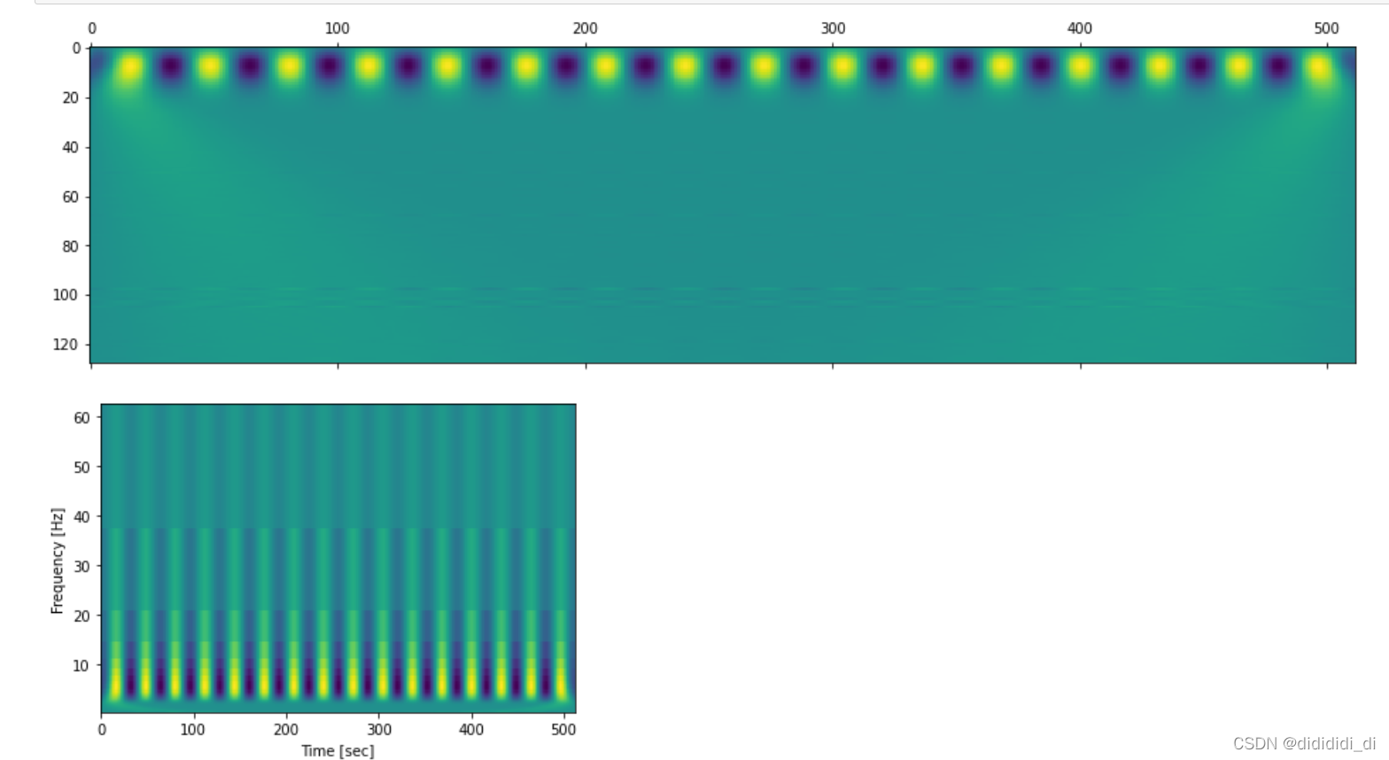
下面是官方的程序的结果及其对比

import pywt
import numpy as np
import matplotlib.pyplot as plt
x = np.arange(512)
y = np.sin(2*np.pi*x/32)
coef, freqs=pywt.cwt(y,np.arange(1,129),'gaus1',1/250)
plt.matshow(coef) # doctest: +SKIP
plt.show() # doctest: +SKIP
plt.pcolormesh(x, freqs, coef)
plt.ylabel('Frequency [Hz]')
plt.xlabel('Time [sec]')
plt.show()

一个用途：

对奇异性比较敏感，可以用于波峰波谷的检测
多多查阅官方文档，对于小波函数的使用方法和用途
参考链接
https://pywavelets.readthedocs.io/en/latest/ref/cwt.html?highlight=cwt
原理参考链接
https://blog.csdn.net/kobeyu652453/article/details/106363835

dwt idwt

离散小波变换和重构
参考链接
https://blog.csdn.net/hnxyxiaomeng/article/details/53122204

小波包分解

小波滤波

关于fft 的理解

（应该是个很简单的东西，但我反复去理解过几遍）
我们从官方给出的例子去看

import numpy as np
from scipy.fftpack import fft,ifft
import matplotlib.pyplot as plt
import seaborn
#采样点选择1400个，因为设置的信号频率分量最高为600赫兹，根据采样定理知采样频率要大于信号频率2倍，所以这里设置采样频率为1400赫兹（即一秒内有1400个采样点，一样意思的）
x=np.linspace(0,1,1400) 
 
#设置需要采样的信号，频率分量有180，390和600
y=7*np.sin(2*np.pi*180*x) + 2.8*np.sin(2*np.pi*390*x)+5.1*np.sin(2*np.pi*600*x)
 
yy=fft(y)      #快速傅里叶变换
yreal = yy.real    # 获取实数部分
yimag = yy.imag    # 获取虚数部分
 
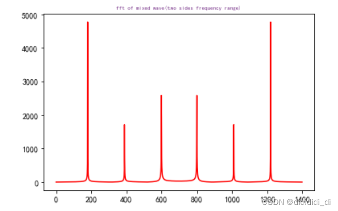
yf=abs(fft(y))    # 取绝对值
yf1=abs(fft(y))/len(x)   #归一化处理
yf2 = yf1[range(int(len(x)/2))] #由于对称性，只取一半区间
 
xf = np.arange(len(y))  # 频率
xf1 = xf
xf2 = xf[range(int(len(x)/2))] #取一半区间
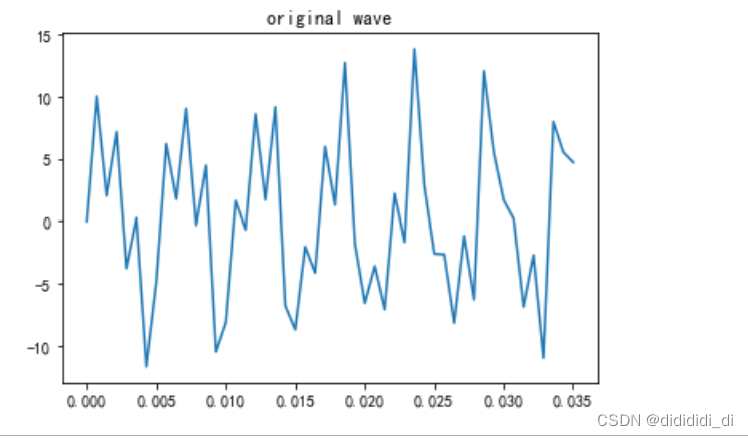
plt.plot(x[0:50],y[0:50])
plt.title('original wave')
plt.show()
plt.plot(xf,yf,'r')
plt.title('fft of mixed wave(two sides frequency range)',fontsize=7,color='#7a378b') #注意这里的颜色可以查询颜色代码表
plt.show()
plt.plot(xf1,yf1,'g')
plt.title('fft of mixed wave(normalization)',fontsize=9,color='r')
plt.show()
plt.plot(xf2,yf2,'b')
plt.title('fft of mixed wave)',fontsize=10,color='#f08080')
plt.show()

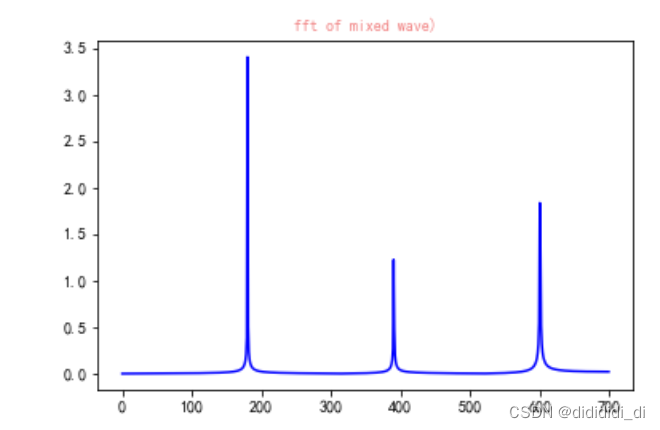
fft 变换不像小波，它是时频对应的，fft仅仅是信号对应的频谱和相位谱，其中幅值是fft结果，其中频率对应的是， 需要进行归一化，是对称的，一般只取一边即可.

Fre = np.arange(int(N/2))*Fs/N  

对应频带

import numpy as np
from scipy.fftpack import fft
import matplotlib.pyplot as plt
Fs =10e3      # 采样频率
f1 =390       # 信号频率1
f2 = 2e3      # 信号频率2
t=np.linspace(0,1,Fs)   # 生成 1s 的实践序列   
noise1 = np.random.random(10e3)      # 0-1 之间的随机噪声
noise2 = np.random.normal(1,10,10e3)
#产生的是一个10e3的高斯噪声点数组集合（均值为：1，标准差：10）
y=2*np.sin(2*np.pi*f1*t)+5*np.sin(2*np.pi*f2*t)+noise2

def FFT (Fs,data):
    L = len (data)                        # 信号长度
    N =np.power(2,np.ceil(np.log2(L)))    # 下一个最近二次幂
    FFT_y1 = np.abs(fft(data,N))/L*2      # N点FFT 变化,但处于信号长度
    Fre = np.arange(int(N/2))*Fs/N        # 频率坐标
    FFT_y1 = FFT_y1[range(int(N/2))]      # 取一半
    return Fre, FFT_y1

Fre, FFT_y1 = FFT(Fs,y)
plt.figure
plt.plot(Fre,FFT_y1)
plt.grid()
plt.show()

相关链接
https://zhuanlan.zhihu.com/p/70347734
http://www.zzvips.com/article/148868.html