机器学习实战—— Chap08.Regression

Linear Regression

import matplotlib.pyplot as plt
import numpy as np

"""
Desc:
    加载数据

Parameters:
    filename - 文件名
    
Returns:
    xArr - x数据集
    yArr - y数据集
"""
def loadDataSet(filename):
    # 计算特征个数，由于最后一列为y值所以减一
    numFeat = len(open(filename).readline().split('\t')) - 1
    xArr = []
    yArr = []
    fr = open(filename)
    for line in fr.readlines():
        lineArr = []
        curLine = line.strip().split('\t')
        for i in range(numFeat):
            lineArr.append(float(curLine[i]))
        xArr.append(lineArr)
        yArr.append(float(curLine[-1]))
    return xArr, yArr


"""
Desc:
    计算回归系数w

Parameters:
    xArr - x数据集
    yArr - y数据集
    
Returns:
    ws - 回归系数
"""
def standRegres(xArr, yArr):
    xMat = np.mat(xArr)
    yMat = np.mat(yArr).T
    xTx = xMat.T * xMat
    # 求矩阵的行列式
    if np.linalg.det(xTx) == 0.0:
        print("矩阵为奇异矩阵，不能求逆")
        return
    # .I求逆矩阵
    ws = (xTx.I) * (xMat.T) * yMat
    return ws


"""
Desc:
    绘制数据集

Parameters:
    None
    
Returns:
    None
"""
def plotDataSet():
    xArr, yArr = loadDataSet('ex0.txt')
    ws = standRegres(xArr, yArr)
    xMat = np.mat(xArr)
    yMat = np.mat(yArr)
    xCopy = xMat.copy()
    # 排序
    xCopy.sort(0)
    yHat = xCopy * ws
    # 以下两行是通过corrcoef函数比较预测值和真实值的相关性
    # corrcoef函数得到相关系数矩阵
    # 得到的结果中对角线上的数据是1.0，因为yMat和自己的匹配是完美的
    # 而yHat1和yMat的相关系数为0.98
    yHat1 = xMat * ws
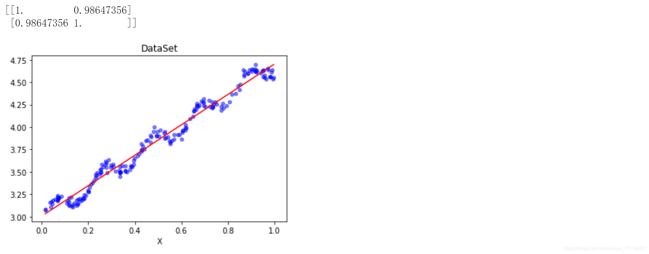
    print(np.corrcoef(yHat1.T, yMat))
    fig = plt.figure()
    ax = fig.add_subplot(111)
    ax.plot(xCopy[:, 1], yHat, c='red')
    # 绘制样本点即
    # flatten返回一个折叠成一维的数组。但是该函数只能适用于numpy对象，即array或者mat，普通的list列表是不行的
    # 矩阵.A(等效于矩阵.getA())变成了数组
    ax.scatter(xMat[:, 1].flatten().A[0], yMat.flatten().A[0], s=20, c='blue', alpha=.5)
    plt.title('DataSet')
    plt.xlabel('X')
    plt.show()
    
    
if __name__ == '__main__':
    plotDataSet()
    

from matplotlib.font_manager import FontProperties
import matplotlib.pyplot as plt
import numpy as np

"""
Desc:
    加载数据

Parameters:
    filename - 文件名
    
Returns:
    xArr - x数据集
    yArr - y数据集
"""
def loadDataSet(filename):
    # 计算特征个数，由于最后一列为y值所以减一
    numFeat = len(open(filename).readline().split('\t')) - 1
    xArr = []
    yArr = []
    fr = open(filename)
    for line in fr.readlines():
        lineArr = []
        curLine = line.strip().split('\t')
        for i in range(numFeat):
            lineArr.append(float(curLine[i]))
        xArr.append(lineArr)
        yArr.append(float(curLine[-1]))
    return xArr, yArr


"""
Desc:
    使用局部加权线性回归计算回归系数w

Parameters:
    testPoint - 测试样本点
    xArr - x数据集
    yArr - y数据集
    k - 高斯核的k，自定义参数
    
Returns:
    ws - 回归系数
"""
def lwlr(testPoint, xArr, yArr, k=1.0):
    xMat = np.mat(xArr)
    yMat = np.mat(yArr).T
    m = np.shape(xMat)[0]
    # 创建加权对角阵
    weights = np.mat(np.eye((m)))
    for j in range(m):
        # 高斯核
        diffMat = testPoint - xMat[j, :]
        weights[j, j] = np.exp(diffMat * diffMat.T / (-2.0 * k**2))
    xTx = xMat.T * (weights * xMat)
    # 求矩阵的行列式
    if np.linalg.det(xTx) == 0.0:
        print("矩阵为奇异矩阵，不能求逆")
        return
    # .I求逆矩阵
    ws = (xTx.I) * (xMat.T * (weights * yMat))
    return testPoint * ws


"""
Desc:
    局部加权线性回归测试

Parameters:
    testArr - 测试数据集
    xArr - x数据集
    yArr - y数据集
    k - 高斯核的k,自定义参数
    
Returns:
    ws - 回归系数
"""
def lwlrTest(testArr, xArr, yArr, k=1.0):
    m = np.shape(testArr)[0]
    yHat = np.zeros(m)
    for i in range(m):
        yHat[i] = lwlr(testArr[i], xArr, yArr, k)
    return yHat


"""
Desc:
    绘制多条局部加权回归曲线

Parameters:
    None
    
Returns:
    None
"""
def plotlwlrRegression():
    # 设置中文字体
    font = FontProperties(fname=r"C:\Windows\Fonts\simsun.ttc", size=14)
    xArr, yArr = loadDataSet('ex0.txt')
    yHat_1 = lwlrTest(xArr, xArr, yArr, 1.0)
    yHat_2 = lwlrTest(xArr, xArr, yArr, 0.01)
    yHat_3 = lwlrTest(xArr, xArr, yArr, 0.003)
    xMat = np.mat(xArr)
    yMat = np.mat(yArr)
    # 排序，返回索引值
    srtInd = xMat[:, 1].argsort(0)
    xSort = xMat[srtInd][:, 0, :]
    fig, axs = plt.subplots(nrows=3, ncols=1, sharex=False, sharey=False, figsize=(10, 8))
    axs[0].plot(xSort[:, 1], yHat_1[srtInd], c='red')
    axs[1].plot(xSort[:, 1], yHat_2[srtInd], c='red')
    axs[2].plot(xSort[:, 1], yHat_3[srtInd], c='red')
    axs[0].scatter(xMat[:, 1].flatten().A[0], yMat.flatten().A[0], s=20, c='blue', alpha=.5)
    axs[1].scatter(xMat[:, 1].flatten().A[0], yMat.flatten().A[0