适合于图像重建问题的归一化层：GENERALIZED NORMALIZATION TRANSFORMATION(GDN)

最新推荐文章于 2024-02-06 17:59:30 发布

ch ur h

最新推荐文章于 2024-02-06 17:59:30 发布

阅读量5.9k

点赞数 18

分类专栏：图像压缩 pytorch 文章标签： pytorch 图像生成图像重建归一化层 GDN

本文链接：https://blog.csdn.net/weixin_41786536/article/details/100547726

版权

pytorch 同时被 2 个专栏收录

12 篇文章 3 订阅

订阅专栏

图像压缩

5 篇文章 6 订阅

订阅专栏

BN层在生成模型中的问题

在一般的卷积神经网络中，batch normalization（BN）批标准化是一种常见的中间处理层，它使得图像均值为0，标准差为1，这样就接近于高斯分布，更符合图像的特征。此外还可以加速训练。
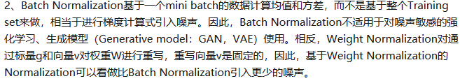
BN层有一个优势，就是每次处理的批量的均值和标准差都不会相同，所以这相当于加入了噪声，增强了模型的泛化能力，但对于图像超分辨率重建、图像生成、图像去噪和图像压缩等生成模型，就不友好了，生成的图像要求尽可能清晰，不应该引入噪声，所以这些应用场景下不应该使用BN层。：知乎上有大神对这个问题的讨论
这里引用lqfarmer大神的回答。
在这里插入图片描述

GDN层

ICLR2016论文《DENSITY MODELING OF IMAGES USING A
GENERALIZED NORMALIZATION TRANSFORMATION》提出了GDN层，是一种更适合图像重建的归一化层。并且作者在ICLR2017论文《END-TO-END OPTIMIZED IMAGE COMPRESSION》中的图像压缩算法中使用了GDN层。

核心公式如下：
$y_{i}=\frac{x_{i}}{(\beta^{2}_{i}+\sum \gamma_{i}\times x_{i}^{2})^{\frac{1}{2}}}$

其中 $x_{i}$ 为第i层的输入特征图， $\beta_{i}$ 和 $\gamma_{i}$ 均为需要学习的参数，这一点与BN层一样。在第一篇论文中，原本这个指数是需要指定的超参数，但是第二篇轮以及以后的论文都默认为2。
这是github上找到的一个GDN层的pytorch实现，以其为例详解其计算过程。
设置初始值 $\beta_{min}=10^{-6}$ , $\gamma_{init}=0.1$ ，偏差 $b=2^{-18}$ , $c h$ 代表这一层的通道数
$\beta_{bound}=[\beta_{min}+b^{2}]^{\frac{1}{2}}$

$\gamma_{bound}=b$

$\beta=(\underbrace{[1,1,\cdots ,1]}_{数量:ch，类型:tensor}+b^{2})^{\frac{1}{2}}$

$\gamma=(\gamma_{init}\times \begin{bmatrix} 1 & 0 & \cdots & 0 \\ 0 & 1 & \cdots & 0 \\ \vdots & \vdots & \ddots & \vdots \\ 0 & 0 & \cdots & 1 \\ \end{bmatrix}_{ch\times ch}+b^{2})^{\frac{1}{2}}$
$\beta=max(\beta,(\underbrace{[1,1,\cdots,1]}_{数量:ch}\times\beta_{bound}))$

以这个 $\beta$ 来进行反向传播学习，然后
$\beta=\beta^{2}-b^{2}$

$\gamma=max(\gamma,( \begin{bmatrix} 1 & 1 & \cdots & 1 \\ 1 & 1 & \cdots & 1 \\ \vdots&\vdots&\ddots&\vdots \\ 1&1&\cdots&1 \\ \end {bmatrix}_ {ch \times ch}\times\gamma_{bound}))$

以这个 $\gamma$ 来进行反向传播学习，然后
$\gamma=\gamma^{2}-b^{2}$

将 $\gamma$ 整形为 $(c h, c h, 1, 1)$ 的形状，相当于核长为1，通道数为 $c h$ 的卷积核，且个数为 $c h$ 。
将这个卷积核作用在输入特征图的平方上，加上偏置 $\beta$ ，就巧妙地完成了 $(\beta^{2}_{i}+\sum \gamma_{i}\times x_{i}^{2})$ 的计算。最后一步：
$y_{i}=\frac{x_{i}}{(\beta_{i}+\sum \gamma_{i}\times x_{i}^{2})^{\frac{1}{2}}}$

代码如下：

import torch
import torch.utils.data
from torch import nn, optim
from torch.nn import functional as F
from torchvision import datasets, transforms
from torchvision.utils import save_image
from torch.autograd import Function


class LowerBound(Function):
    def forward(ctx, inputs, bound):
        b = torch.ones(inputs.size())*bound
        b = b.to(inputs.device)
        ctx.save_for_backward(inputs, b)
        return torch.max(inputs, b)
  
    def backward(ctx, grad_output):
        inputs, b = ctx.saved_tensors

        pass_through_1 = inputs >= b
        pass_through_2 = grad_output < 0

        pass_through = pass_through_1 | pass_through_2
        return pass_through.type(grad_output.dtype) * grad_output, None


class GDN(nn.Module):
    """Generalized divisive normalization layer.
    y[i] = x[i] / sqrt(beta[i] + sum_j(gamma[j, i] * x[j]))
    """
  
    def __init__(self,
                 ch,
                 device,
                 inverse=False,
                 beta_min=1e-6,
                 gamma_init=.1,
                 reparam_offset=2**-18):
        super(GDN, self).__init__()
        self.inverse = inverse
        self.beta_min = beta_min
        self.gamma_init = gamma_init
        self.reparam_offset = torch.FloatTensor([reparam_offset])

        self.build(ch, torch.device(device))
  
    def build(self, ch, device):
        self.pedestal = self.reparam_offset**2
        self.beta_bound = (self.beta_min + self.reparam_offset**2)**.5
        self.gamma_bound = self.reparam_offset
  
        # Create beta param
        beta = torch.sqrt(torch.ones(ch)+self.pedestal)
        self.beta = nn.Parameter(beta.to(device))

        # Create gamma param
        eye = torch.eye(ch)
        g = self.gamma_init*eye
        g = g + self.pedestal
        gamma = torch.sqrt(g)

        self.gamma = nn.Parameter(gamma.to(device))
        self.pedestal = self.pedestal.to(device)

    def forward(self, inputs):
        device_id = inputs.device.index

        beta = self.beta.to(device_id)
        gamma = self.gamma.to(device_id)
        pedestal = self.pedestal.to(device_id) 

        unfold = False
        if inputs.dim() == 5:
            unfold = True
            bs, ch, d, w, h = inputs.size() 
            inputs = inputs.view(bs, ch, d*w, h)

        _, ch, _, _ = inputs.size()

        # Beta bound and reparam
        beta = LowerBound()(beta, self.beta_bound)
        beta = beta**2 - pedestal 

        # Gamma bound and reparam
        gamma = LowerBound()(gamma, self.gamma_bound)
        gamma = gamma**2 - pedestal
        gamma  = gamma.view(ch, ch, 1, 1)

        # Norm pool calc
        norm_ = nn.functional.conv2d(inputs**2, gamma, beta)
        norm_ = torch.sqrt(norm_)

        # Apply norm
        if self.inverse:
            outputs = inputs * norm_
        else:
            outputs = inputs / norm_

        if unfold:
            outputs = outputs.view(bs, ch, d, w, h)
        return outputs

将其命名为pytorch_gdn.py，在自己的模型中导入即可

from pytorch_gdn import GDN
......
class net(nn.Module):

    def __init__(self):
        super(net,self).__init__()
        ......
		device = torch.device('cuda')
		
		self.gdn = GDN(ch, device)#ch为这一层的通道数
	def forward(self,input):
        ......
        self.output = self.gdn(self.output)
        ......
        return self.output